Typst Examples Book
This book provides an extended tutorial and lots of Typst snippets that can help you to write better Typst code.
However, all of them should compile on last version of Typst1.
CAUTION: the book is (probably forever) a WIP, so don't rely on it.
If you like it, consider giving a star on GitHub!
This will help me to stay motivated and continue working on this book.
Navigation
The book consists of several chapters, each with its own goal:
Contributions
Any contributions are very welcome! If you have a good code snippet that you want to share, feel free to submit an issue with snippet or make a PR in the repository.
I will especially appreciate submissions of active community members and compiler contributors!
However, I will also really appreciate feedback from beginners to make the book as comprehensible as possible!
Acknowledgements
Thanks to everyone in the community who published their code snippets!
If someone doesn't like their code and/or name being published, please contact me.
When a new version launches, it may take some time to update the book, feel free to tag me to speed up the process.
Getting started
Typst is an open-source project that can be built into a pretty small binary, that is very easy to install or even use in Web. Typst is managed and built by a company, a company, the main product of which is Typst editing Web App.
So there are two possibilities for working with Typst: use online Web App or install Typst locally and work with it from your favorite editor. I will briefly cover these two ways with their pros and cons in this chapter.
WebApp
Starting is pretty simple: sign on typst.app and create a new document. Then... Just start typing, and the document with your text will appear in the preview Panel.
I highly recommend starting from scratch at first to try things. When you get some better understanding on Typst, you can continue with templates, instructions to style your document ready-to-use. But even then, sometimes it is just easier to make all you need exactly as you need from scratch. Typst makes it easy.
Pros:
- Very easy to start
- Perfect for collaboration.
- Features: Typst Team has put lots of effort into the app, so it has a lot of pretty good features (like smart dictionary check or Vim keybindings for pros).
- Working Offline: Once the page is loaded, you can go offline. Compiling document is done on your computer, so you don't need internet connection to make it. And all changes will be saved locally.
- Easy to work with same projects across devices.
- Comes with even more cool features at their paid plan, Typst Pro: like comments for collaboration and Github sync.
It's also a pretty good opportunity to support the project (though there are other ways to support them, like Github Sponsors, contributing and spreading the word about Typst
:)).
Cons:
- Still requires internet
- Your data is stored online, your development (however, you can make backups and the app crashes very rarely)
- The App lacks some features that are present in local editors and Tinymist LSP.
- With local compiler, you can do pretty wild automations, like making automatic report generators.
Local development
Tinymist
Don't use Typst LSP, that's a very outdated thing.
Tinymist is a community-developed LSP 1 that probably has even more features than Web App (well, that may change in some time, and I'm not known for keeping this book very up-to-date). These include things like going-to-defenition, refactoring, formatting,, opening packages the errors are comming from and many-many others. It's not "official", but it doesn't make it any worse. It is definitely worth trying.
Works with pretty much any editor supporting LSP. For VS Cod(e,ium), Neovim, Emacs, Sublime Text, Helix and Zed there are also useful frontends available.
So, to use Typst locally, it's probably enough to open your favourite editor, install Tinymist extension and get a full Typst experience with live preview and many other nice things.
Tinymist uses Typst as a library, so it comes with it's own inner Typst version. Sometimes, for example, if your VS Code version is too old, it can't install newer version, and you end up with old Typst version without knowing it.
Oh, yep, Tinymist can export documents in any needed format, by the way. You can also set up it to do it automatically on save, too.
And it's actually possible to just use
tinymist preview document.typfrom terminal, if it's a properly installed tool (that would open a browser preview).
Pros:
- Features: probably the largest set available for Typst.
- Best for programmers or experienced users.
- It's just a LSP, all other things you need come from your editor, system and so on. It's easy to work with Github, easy to integrate it in whatever you want.
Cons:
- It's probably a bit harder than just launching WebApp.
- Collaborating that way is much harder. It requires using Github or setting up your editor.
- Worse portability (you have to sync your files).
- There are tiny chances that the development will be dropped in future.
CLI
Typst also comes with it's own CLI (command-line-tool). This way, it is enough to install on your system and then launch from terminal typst c your_file.typ (or compile instead of c) to get a PDF, compiled from your your_file.typ document.
Installation notes:
- Windows users: just download the exe from Github Releases and unpack it somewhere in your PATH
- Unix users: https://github.com/typst/typst?tab=readme-ov-file#installation. Note: Typst version sometimes significantly lags at package managers (and it's not Typst' fault).
This way, you can open your favorite text editor, like Notepad (or Vim without any plugins), write Typst document there, then compiling it and looking at the result.
CLI also supports watching file: typst w your_file.typ (or watch instead of w). That way, Typst will recompile it each time it is changed (and saved).
That way, however, I recommend having a live preview PDF viewer, that would update the viewed PDF as it is changed with need for reload.
These include:
- SumatraPDF (works on Windows)
- Zathura and Sioyek (Linux)
- Okular (cross-platform)
- MuPDF (must be combined with
entron Unix) - (some others I've forgotten, feel free to make an Issue / PR)
(note that it is not perfect, there probably would be some blinking, but it's much better than having to reload)
Pros:
- Perfect for "I need to quickly compile this file". You can use it along with Tinymist, using Tinymist for preview and editing, and CLI for the fast and precise exporting.
- Perfect for complex automations and using it from other apps.
- Can self-update for required version with one command (if installed not from package manager)
Cons:
- Harder to use
- Doesn't provide editor features
Let's go
I hope you have managed to get something working, so let's go diving into Typst!
A language-server protocol, a thing that provides cool things like autocompletion or refactoring features for most editors.
Typst Basics
This is a chapter that consistently introduces you to the most things you need to know when writing with Typst.
It show much more things than official tutorial, so maybe it will be interesting to read for some of the experienced users too.
Some examples are taken from Official Tutorial and Official Reference. Most are created and edited specially for this book.
Important: in most cases there will be used "clipped" examples of your rendered documents (no margins, smaller width and so on).
To set up the spacing as you want, see Official Page Setup Guide.
Tutorial by Examples
The first section of Typst Basics is very similar to Official Tutorial, with more specialized examples and less words. It is highly recommended to read the official tutorial anyway.
Markup language
Starting
Starting typing in Typst is easy.
You don't need packages or other weird things for most of things.

Blank line will move text to a new paragraph.

Btw, you can use any language and unicode symbols
without any problems as long as the font supports it: ßçœ̃ɛ̃ø∀αβёыა😆…
Markup
= Markup

This was a heading. Number of `=` in front of name corresponds to heading level.

== Second-level heading

Okay, let's move to _emphasis_ and *bold* text.

Markup syntax is generally similar to
`AsciiDoc` (this was `raw` for monospace text!)
New lines & Escaping
You can break \
line anywhere you \
want using "\\" symbol.

Also you can use that symbol to
escape \_all the symbols you want\_,
if you don't want it to be interpreted as markup
or other special symbols.
Comments & codeblocks
You can write comments with `//` and `/* comment */`:
// Like this
/* Or even like
this */

```typ
Just in case you didn't read source,
this is how it is written:

// Like this
/* Or even like
this */

By the way, I'm writing it all in a _fenced code block_ with *syntax highlighting*!
```
Smart quotes
== What else?

There are not much things in basic "markup" syntax,
but we will see much more interesting things very soon!
I hope you noticed auto-matched "smart quotes" there.
Lists
- Writing lists in a simple way is great.
- Nothing complex, start your points with `-`
  and this will become a list.
  - Indented lists are created via indentation.

+ Numbered lists start with `+` instead of `-`.
+ There is no alternative markup syntax for lists
+ So just remember `-` and `+`, all other symbols
  wouldn't work in an unintended way.
  + That is a general property of Typst's markup.
  + Unlike Markdown, there is only one way
    to write something with it.
Notice:
Typst numbered lists differ from markdown-like syntax for lists. If you write them by hand, numbering is preserved:

1. Apple
1. Orange
1. Peach
Math
I will just mention math ($a + b/c = sum_i x^i$)
is possible and quite pretty there:

$
7.32 beta +
  sum_(i=0)^nabla
    (Q_i (a_i - epsilon)) / 2
$

To learn more about math, see corresponding chapter.
Functions
Functions
Okay, let's now move to more complex things.

A major part of Typst's magic is its scripting.
To enter scripting mode, type `#` and then a *function name*
after that. We will start with _something dull_:

#lorem(50)

_That *function* just generated 50 "Lorem Ipsum" words!_
More functions
#underline[functions can do everything!]

#text(orange)[L]ike #text(size: 0.8em)[Really] #sub[E]verything!

#figure(
  caption: [
    This is a screenshot from one of first theses written in Typst. \
    _All these things are written with #text(blue)[custom functions] too._
  ],
  image("../boxes.png", width: 80%)
)

In fact, you can #strong[forget] about markup
and #emph[just write] functions everywhere!

#list[
  All that markup is just a #emph[syntax sugar] over functions!
]
How to call functions
First, start with `#`. Then write the name.
Finally, write some parentheses and maybe something inside.

You can navigate lots of built-in functions
in #link("https://typst.app/docs/reference/")[Official Reference].

#quote(block: true, attribution: "Typst Examples Book")[
  That's right, links, quotes and lots of
  other document elements are created with functions.
]
Function arguments
There are _two types_ of function arguments:

+ *Positional.* Like `50` in `lorem(50)`.
  Just write them in parentheses and it will be okay.
  If you have many, use commas.
+ *Named.* Like in `#quote(attribution: "Whoever")`.
  Write the value after a name and a colon.

If argument is named, it has some _default value_.
To find out what it is, see
#link("https://typst.app/docs/reference/")[Official Typst Reference].
Content
Now we should probably try writing our own functions
The most "universal" type in Typst language is *content*.
Everything you write in the document becomes content.

#[
  But you can explicitly create it with
  _scripting mode_ and *square brackets*.

  There, in square brackets, you can use any markup
  functions or whatever you want.
]
Markup and code modes
When you use `#`, you are "switching" to code mode.
When you use `[]`, you turn back into _markup_ (or content) mode:

// +-- going from markup (the default mode) to scripting for that function
// |                 +-- scripting mode: calling `text`, the last argument is markup
// |     first arg   |
// v     vvvvvvvvv   vvvv
   #rect(width: 5cm, text(red)[hello *world*])
//  ^^^^                       ^^^^^^^^^^^^^ just a markup argument for `text`
//  |
//  +-- calling `rect` in scripting mode, with two arguments: width and other content
Passing content into functions
So what are these square brackets after functions?

If you *write content right after
function, it will be passed as positional argument there*.

#quote(block: true)[
  So #text(red)[_that_] allows me to write
  _literally anything in things
  I pass to #underline[functions]!_
]
Passing content, part II
So, just to make it clear, when I write

```typ
- #text(red)[red text]
- #text([red text], red)
- #text("red text", red)
//      ^        ^
// Quotes there mean a plain string, not a content!
// This is just text.
```

It all will result in a #text([red text], red).
Cheatsheet
Here is a brief cheetsheet for some most needed Typst concepts (by @mewmew and @7i):

Basic styling
Set rule
#set page(width: 15cm, margin: (left: 4cm, right: 4cm))

That was great, but using functions everywhere, especially
with many arguments every time is awfully cumbersome.

That's why Typst has _rules_. No, not for you, for the document.

#set par(justify: true)

And the first rule we will consider there is `set` rule.
As you see, I've just used it on `par` (which is short from paragraph)
and now all paragraphs became _justified_.

It will apply to all paragraphs after the rule,
but will work only in its _scope_ (we will discuss them later).

#par(justify: false)[
  Of course, you can override a `set` rule.
  This rule just sets the _default value_
  of an argument of an element.
]

By the way, at first line of this snippet
I've reduced page size to make justifying more visible,
also increasing margins to add blank space on left and right.
A bit about length units
Before we continue with rules, we should talk about length. There are several absolute length units in Typst:

#set rect(height: 1em)

#table(
  columns: 2,
  [Points], rect(width: 72pt),
  [Millimeters], rect(width: 25.4mm),
  [Centimeters], rect(width: 2.54cm),
  [Inches], rect(width: 1in),
  [Relative to font size], rect(width: 6.5em)
)

`1 em` = current font size. \
It is a very convenient unit,
so we are going to use it a lot
Setting something else
Of course, you can use set rule with all built-in functions
and all their named arguments to make some argument "default".
For example, let's make all quotes in this snippet authored by the book:
#set quote(block: true, attribution: [Typst Examples Book])

#quote[
  Typst is great!
]

#quote[
  The problem with quotes on the internet is
  that it is hard to verify their authenticity.
]
Opinionated defaults
That allows you to set Typst default styling as you want it:
#set par(justify: true)
#set list(indent: 1em)
#set enum(indent: 1em)
#set page(numbering: "1")

- List item
- List item

+ Enum item
+ Enum item
Don't complain about bad defaults! Set your own.
Numbering
= Numbering

Some of elements have a property called "numbering".
They accept so-called "numbering patterns" and
are very useful with set rules. Let's see what I mean.

#set heading(numbering: "I.1:")

= This is first level
= Another first
== Second
== Another second
=== Now third
== And second again
= Now returning to first
= These are actual roman numerals
Of course, there are lots of other cool properties that can be set, so feel free to dive into Official Reference and explore them!
And now we are moving into something much more interesting…
Advanced styling
The show rule
Advanced styling comes with another rule. The _`show` rule_.

Now please compare the source code and the output.

#show "Be careful": strong[Play]

This is a very powerful thing, sometimes even too powerful.
Be careful with it.

#show "it is holding me hostage": text(green)[I'm fine]

Wait, what? I told you "Be careful!", not "Play!".

Help, it is holding me hostage.
Now a bit more serious
Show rule is a powerful thing that takes a _selector_
and what to apply to it. After that it will apply to
all elements it can find.

It may be extremely useful like that:

#show emph: set text(blue)

Now if I want to _emphasize_ something,
it will be both _emphasized_ and _blue_.
Isn't that cool?
About syntax
Sometimes show rules may be confusing. They may seem very diverse, but in fact they all are quite the same! So

// actually, this is the same as
// redify = text.with(red)
// `with` creates a new function with that argument already set
#let redify(string) = text(red, string)

// and this is the same as
// framify = rect.with(stroke: orange)
#let framify(object) = rect(object, stroke: orange)

// set default color of text blue for all following text
#show: set text(blue)

Blue text.

// wrap everything into a frame
#show: framify

Framed text.

// it's the same, just creating new function that calls framify
#show: a => framify(a)

Double-framed.

// apply function to `the`
#show "the": redify
// set text color for all the headings
#show heading: set text(purple)

= Conclusion

All these rules are doing basically the same thing!
Blocks
One of the most important usages is that you can set up all spacing using blocks. Like every element with text contains text that can be set up, every block element contains blocks:
Text before
= Heading
Text after

#show heading: set block(spacing: 0.5em)

Text before
= Heading
Text after
Selector
So show rule can accept _selectors_.

There are lots of different selector types,
for example

- element functions
- strings
- regular expressions
- field filters

Let's see example of the latter:

#show heading.where(level: 1): set align(center)

= Title
== Small title

Of course, you can set align by hand,
no need to use show rules
(but they are very handy!):

#align(center)[== Centered small title]
Custom formatting
Let's try now writing custom functions.
It is very easy, see yourself:

// "it" is a heading, we take it and output things in braces
#show heading: it => {
  // center it
  set align(center)
  // set size and weight
  set text(12pt, weight: "regular")
  // see more about blocks and boxes
  // in corresponding chapter
  block(smallcaps(it.body))
}

= Smallcaps heading

Setting spacing
TODO: explain block spacing for common elements
Formatting to get an "article look"
#set page(
  // Header is that small thing on top
  header: align(
    right + horizon,
    [Some header there]
  ),
  height: 12cm
)

#align(center, text(17pt)[
  *Important title*
])

#grid(
  columns: (1fr, 1fr),
  align(center)[
    Some author \
    Some Institute \
    #link("mailto:some@mail.edu")
  ],
  align(center)[
    Another author \
    Another Institute \
    #link("mailto:another@mail.edu")
  ]
)

Now let's split text into two columns:

#show: rest => columns(2, rest)

#show heading.where(
  level: 1
): it => block(width: 100%)[
  #set align(center)
  #set text(12pt, weight: "regular")
  #smallcaps(it.body)
]

#show heading.where(
  level: 2
): it => text(
  size: 11pt,
  weight: "regular",
  style: "italic",
  it.body + [.],
)

// Now let's fill it with words:

= Heading
== Small heading
#lorem(10)
== Second subchapter
#lorem(10)
= Second heading
#lorem(40)

== Second subchapter
#lorem(40)
Templates
Templates
If you want to reuse styling in other files, you can use the template idiom.
Because set and show rules are only active in their current scope, they
will not affect content in a file you imported your file into. But functions
can circumvent this in a predictable way:
// define a function that:
// - takes content
// - applies styling to it
// - returns the styled content
#let apply-template(body) = [
  #show heading.where(level: 1): emph
  #set heading(numbering: "1.1")
  // ...
  #body
]
This is equivalent to:
// we can reduce the number of hashes needed here by using scripting mode
// same as above but we exchanged `[...]` for `{...}` to switch from markup
// into scripting mode
#let apply-template(body) = {
  show heading.where(level: 1): emph
  set heading(numbering: "1.1")
  // ...
  body
}
Then in your main file:
#import "template.typ": apply-template
#show: apply-template
This will apply a "template" function to the rest of your document!
Passing arguments
// add optional named arguments
#let apply-template(body, name: "My document") = {
  show heading.where(level: 1): emph
  set heading(numbering: "1.1")

  align(center, text(name, size: 2em))

  body
}
Then, in template file:
#import "template.typ": apply-template

// `func.with(..)` applies the arguments to the function and returns the new
// function with those defaults applied
#show: apply-template.with(name: "Report")

// it is functionally the same as this
#let new-template(..args) = apply-template(name: "Report", ..args)
#show: new-template
Writing templates is fairly easy if you understand scripting.
See more information about writing templates in Official Tutorial.
There is no official repository for templates yet, but there are a plenty community ones in awesome-typst.
Must-know
This section contains things, that are not general enough to be part of "tutorial", but still are very important to know for proper typesetting.
Feel free to skip through things you are sure you will not use.
Boxing & Blocking
You can use boxes to wrap anything
into text: #box(image("../tiger.jpg", height: 2em)).

Blocks will always be "separate paragraphs".
They will not fit into a text: #block(image("../tiger.jpg", height: 2em))
Both have similar useful properties:
#box(stroke: red, inset: 1em)[Box text]
#block(stroke: red, inset: 1em)[Block text]
rect
There is also rect that works like block, but has useful default inset and stroke:
#rect[Block text]
Figures
For the purposes of adding a figure to your document, use figure function. Don't try to use boxes or blocks there.
Figures are that things like centered images (probably with captions), tables, even code.
@tiger shows a tiger. Tigers
are animals.

#figure(
  image("../tiger.jpg", width: 80%),
  caption: [A tiger.],
) <tiger>
In fact, you can put there anything you want:
They told me to write a letter to you. Here it is:

#figure(
  text(size: 5em)[I],
  caption: [I'm cool, right?],
) 
Using spacing
Most time you will pass spacing into functions. There are special function fields that take only size.
They are usually called like width, length, in(out)set, spacing and so on.
Like in CSS, one of the ways to set up spacing in Typst is setting margins and padding of elements.
However, you can also insert spacing directly using functions h (horizontal spacing) and v (vertical spacing).
Horizontal #h(1cm) spacing.
#v(1cm)
And some vertical too!
Absolute length units
Link to reference
Absolute length (aka just "length") units are not affected by outer content and size of parent.
#set rect(height: 1em)
#table(
  columns: 2,
  [Points], rect(width: 72pt),
  [Millimeters], rect(width: 25.4mm),
  [Centimeters], rect(width: 2.54cm),
  [Inches], rect(width: 1in),
)
Relative to current font size
1em = 1 current font size:
#set rect(height: 1em)
#table(
  columns: 2,
  [Centimeters], rect(width: 2.54cm),
  [Relative to font size], rect(width: 6.5em)
)

Double font size: #box(stroke: red, baseline: 40%, height: 2em, width: 2em)
It is a very convenient unit, so it is used a lot in Typst.
Combined
Combined: #box(rect(height: 5pt + 1em))

#(5pt + 1em).abs
#(5pt + 1em).em
Ratio length
Link to reference
1% = 1% from parent size in that dimension
This line width is 50% of available page size (without margins):

#line(length: 50%)

This line width is 50% of the box width: #box(stroke: red, width: 4em, inset: (y: 0.5em), line(length: 50%))
Relative length
Link to reference
You can combine absolute and ratio lengths into relative length:
#rect(width: 100% - 50pt)

#(100% - 50pt).length \
#(100% - 50pt).ratio
Fractional length
Link to reference
Single fraction length just takes maximum size possible to fill the parent:
Left #h(1fr) Right

#rect(height: 1em)[
  #h(1fr)
]
There are not many places you can use fractions, mainly those are h and v.
Several fractions
If you use several fractions inside one parent, they will take all remaining space proportional to their number:
Left #h(1fr) Left-ish #h(2fr) Right
Nested layout
Remember that fractions work in parent only, don't rely on them in nested layout:
Word: #h(1fr) #box(height: 1em, stroke: red)[
  #h(2fr)
]
Placing, Moving, Scale & Hide
This is a very important section if you want to do arbitrary things with layout, create custom elements and hacking a way around current Typst limitations.
TODO: WIP, add text and better examples
Place
Ignore layout, just put some object somehow relative to parent and current position. The placed object will not affect layouting
Link to reference
#set page(height: 60pt)
Hello, world!

#place(
  top + right, // place at the page right and top
  square(
    width: 20pt,
    stroke: 2pt + blue
  ),
)
Basic floating with place
#set page(height: 150pt)
#let note(where, body) = place(
  center + where,
  float: true,
  clearance: 6pt,
  rect(body),
)

#lorem(10)
#note(bottom)[Bottom 1]
#note(bottom)[Bottom 2]
#lorem(40)
#note(top)[Top]
#lorem(10)

dx, dy
Manually change position by (dx, dy) relative to intended.
#set page(height: 100pt)
#for i in range(16) {
  let amount = i * 4pt
  place(center, dx: amount - 32pt, dy: amount)[A]
}
Move
Link to reference
#rect(inset: 0pt, move(
  dx: 6pt, dy: 6pt,
  rect(
    inset: 8pt,
    fill: white,
    stroke: black,
    [Abra cadabra]
  )
))
Scale
Scale content without affecting the layout.
Link to reference
#scale(x: -100%)[This is mirrored.]
A#box(scale(75%)[A])A \
B#box(scale(75%, origin: bottom + left)[B])B
Hide
Don't show content, but leave empty space there.
Link to reference
Hello Jane \
#hide[Hello] Joe
Tables and grids
While tables are not that necessary to know if you don't plan to use them in your documents, grids may be very useful for document layout. We will use both of them them in the book later.
Let's not bother with copying examples from official documentation. Just make sure to skim through it, okay?
Basic snippets
Spreading
Spreading operators (see there) may be especially useful for the tables:
#set text(size: 9pt)

#let yield_cells(n) = {
  for i in range(0, n + 1) {
    for j in range(0, n + 1) {
      let product = if i * j != 0 {
        // math is used for the better look
        if j <= i { $#{ j * i }$ }
        else {
          // upper part of the table
          text(gray.darken(50%), str(i * j))
        }
      } else {
        if i == j {
          // the top right corner
          $times$
        } else {
          // on of them is zero, we are at top/left
          $#{i + j}$
        }
      }
      // this is an array, for loops merge them together
      // into one large array of cells
      (
        table.cell(
          fill: if i == j and j == 0 { orange } // top right corner
          else if i == j { yellow } // the diagonal
          else if i * j == 0 { blue.lighten(50%) }, // multipliers
          product,),
      )
    }
  }
}

#let n = 10
#table(
  columns: (0.6cm,) * (n + 1), rows: (0.6cm,) * (n + 1), align: center + horizon, inset: 3pt, ..yield_cells(n),
)
Highlighting table row
#table(
  columns: 2,
  fill: (x, y) => if y == 2 { highlight.fill },
  [A], [B],
  [C], [D],
  [E], [F],
  [G], [H],
)
For individual cells, use
#table(
  columns: 2,
  [A], [B],
  table.cell(fill: yellow)[C], table.cell(fill: yellow)[D],
  [E], [F],
  [G], [H],
)
Splitting tables
Tables are split between pages automatically.
#set page(height: 8em)
#(
table(
  columns: 5,
  [Aligner], [publication], [Indexing], [Pairwise alignment], [Max. read length  (bp)],
  [BWA], [2009], [BWT-FM], [Semi-Global], [125],
  [Bowtie], [2009], [BWT-FM], [HD], [76],
  [CloudBurst], [2009], [Hashing], [Landau-Vishkin], [36],
  [GNUMAP], [2009], [Hashing], [NW], [36]
  )
)

However, if you want to make it breakable inside other element, you'll have to make that element breakable too:
#set page(height: 8em)
// Without this, the table fails to split upon several pages
#show figure: set block(breakable: true)
#figure(
table(
  columns: 5,
  [Aligner], [publication], [Indexing], [Pairwise alignment], [Max. read length  (bp)],
  [BWA], [2009], [BWT-FM], [Semi-Global], [125],
  [Bowtie], [2009], [BWT-FM], [HD], [76],
  [CloudBurst], [2009], [Hashing], [Landau-Vishkin], [36],
  [GNUMAP], [2009], [Hashing], [NW], [36]
  )
)

Project structure
Large document
Once the document becomes large enough, it becomes harder to navigate it. If you haven't reached that size yet, you can ignore that section.
For managing that I would recommend splitting your document into chapters. It is just a way to work with this, but once you understand how it works, you can do anything you want.
Let's say you have two chapters, then the recommended structure will look like this:
#import "@preview/treet:0.1.1": *

#show list: tree-list
#set par(leading: 0.8em)
#show list: set text(font: "DejaVu Sans Mono", size: 0.8em)
- chapters/
  - chapter_1.typ
  - chapter_2.typ
- main.typ 👁 #text(gray)[← document entry point]
- template.typ
Let's see what to put in each of these files.
Template
In the "template" file goes all useful functions and variables you will use across the chapters. If you have your own template or want to write one, you can write it there.
// template.typ

#let template = doc => {
    set page(header: "My super document")
    show "physics": "magic"
    doc
}

#let infoblock = block.with(stroke: blue, fill: blue.lighten(70%))
#let author = "@sitandr"
Main
This file should be compiled to get the whole compiled document.
// main.typ

#import "template.typ": *
// if you have a template
#show: template

= This is the document title

// some additional formatting

#show emph: set text(blue)

// but don't define functions or variables there!
// chapters will not see it

// Now the chapters themselves as some Typst content
#include("chapters/chapter_1.typ")
#include("chapters/chapter_1.typ")
Chapter
// chapter_1.typ

#import "../template.typ": *

That's just content with _styling_ and blocks:

#infoblock[Some information].

// just any content you want to include in the document
Notes
Note that modules in Typst can see only what they created themselves or imported. Anything else is invisible for them. That's why you need template.typ file to define all functions within.
That means chapters don't see each other either, only what is in the template.
Cyclic imports
Important: Typst forbids cyclic imports. That means you can't import chapter_1 from chapter_2 and chapter_2 from chapter_1 at the same time!
But the good news is that you can always create some other file to import variable from.
Scripting
Typst has a complete interpreted language inside. One of key aspects of working with your document in a nicer way
Basics
Variables I
Let's start with variables.
The concept is very simple, just some value you can reuse:
#let author = "John Doe"

This is a book by #author. #author is a great guy.

#quote(block: true, attribution: author)[
  \<Some quote\>
]
Variables II
You can store any Typst value in variable:
#let block_text = block(stroke: red, inset: 1em)[Text]

#block_text

#figure(caption: "The block", block_text)
Functions
We have already seen some "custom" functions in Advanced Styling chapter.
Functions are values that take some values and output some values:
// This is a syntax that we have seen earlier
#let f = (name) => "Hello, " + name

#f("world!")
Alternative syntax
You can write the same shorter:
// The following syntaxes are equivalent
#let f = (name) => "Hello, " + name
#let f(name) = "Hello, " + name

#f("world!")
Braces, brackets and default
Square brackets
You may remember that square brackets convert everything inside to content.
#let v = [Some text, _markup_ and other #strong[functions]]
#v
We may use same for functions bodies:
#let f(name) = [Hello, #name]
#f[World] // also don't forget we can use it to pass content!
Important: It is very hard to convert content to plain text, as content may contain anything! So be careful when passing and storing content in variables.
Braces
However, we often want to use code inside functions.
That's when we use {}:
#let f(name) = {
  // this is code mode

  // First part of our output
  "Hello, "

  // we check if name is empty, and if it is,
  // insert placeholder
  if name == "" {
      "anonym"
  } else {
      name
  }

  // finish sentence
  "!"
}

#f("")
#f("Joe")
#f("world")
Default values
What we made just now was inventing "default values".
They are very common in styling, so there is a special syntax for them:
#let f(name: "anonym") = [Hello, #name!]

#f()
#f(name: "Joe")
#f(name: "world")
You may have noticed that the argument became named now. In Typst, named argument is an argument that has default value.
When to use brackets and braces
So, as we have seen, we can use both
#let f(name) = [
  Hello, #name
]
#f("Joe")
And
#let f(name) = {
  [Hello,]
  name
}
#f("Joe")
So when to use what?
Well, the answer is simple: which way the code is cleaner.
So don't do that:
// DON'T DO THAT
// PLEASE
#let f(inner) = [
  #set align(center)
  #set box(stroke: red)
  #show heading: it => [
    #set text(size: 2em)
    #it
  ]
  #box[#inner]
]
Can you see how it can be simplified when using code mode?
Scopes
This is a very important thing to remember.
You can't use variables outside of scopes they are defined (unless it is file root, then you can import them). Set and show rules affect things in their scope only.
#{
  let a = 3;
}
// can't use "a" there.

#[
  #show "true": "false"

  This is true.
]

This is true.
Return
Important: by default braces return anything that "returns" into them. For example,
#let change_world() = {
  // some code there changing everything in the world
  str(4e7)
  // another code changing the world
}

#let g() = {
  "Hahaha, I will change the world now! "
  change_world()
  " So here is my long evil monologue..."
}

#g()
To avoid returning everything, return only what you want explicitly, otherwise everything will be joined into one object:
#let f() = {
  "Some long text"
  // Crazy numbers
  "2e7"
  return none
}

// Returns nothing
#f()
Types, part I
Each value in Typst has a type. You don't have to specify it, but it is important.
Content (content)
We have already seen it. A type that represents what is displayed in document.
#let c = [It is _content_!]

// Check type of c
#(type(c) == content)

#c

// repr gives an "inner representation" of value
#repr(c)
Important: It is very hard to convert content to plain text, as content may contain anything! So be careful when passing and storing content in variables.
None (none)
Nothing. Also known as null in other languages. It isn't displayed, converts to empty content.
#none
#repr(none)
String (str)
String contains only plain text and no formatting. Just some chars. That allows us to work with chars:
#let s = "Some large string. There could be escape sentences: \n,
 line breaks, and even unicode codes: \u{1251}"
#s \
#type(s) \
`repr`: #repr(s)

#let s = "another small string"
#s.replace("a", sym.alpha) \
#s.split(" ") // split by space
You can convert other types to their string representation using this type's constructor (e.g. convert number to string):
#str(5) // string, can be worked with as string
Boolean (bool)
true/false. Used in if and many others
#let b = false
#b \
#repr(b) \
#(true and not true or true) = #((true and (not true)) or true) \
#if (4 > 3) {
  "4 is more than 3"
}
Integer (int)
A whole number.
The number can also be specified as hexadecimal, octal, or binary by starting it with a zero followed by either x, o, or b.
#let n = 5
#n \
#(n += 1) \
#n \
#calc.pow(2, n) \
#type(n) \
#repr(n)
#(1 + 2) \
#(2 - 5) \
#(3 + 4 < 8)
#0xff \
#0o10 \
#0b1001
You can convert a value to an integer with this type's constructor (e.g. convert string to int).
#int(false) \
#int(true) \
#int(2.7) \
#(int("27") + int("4"))
Float (float)
Works the same way as integer, but can store floating point numbers. However, precision may be lost.
#let n = 5.0

// You can mix floats and integers,
// they will be implicitly converted
#(n += 1) \
#calc.pow(2, n) \
#(0.2 + 0.1) \
#type(n) 
#3.14 \
#1e4 \
#(10 / 4)
You can convert a value to a float with this type's constructor (e.g. convert string to float).
#float(40%) \
#float("2.7") \
#float("1e5")
Types, part II
In Typst, most of things are immutable. You can't change content, you can just create new using this one (for example, using addition).
Immutability is very important for Typst since it tries to be as pure language as possible. Functions do nothing outside of returning some value.
However, purity is partly "broken" by these types. They are super-useful and not adding them would make Typst much pain.
However, using them adds complexity.
Arrays (array)
Mutable object that stores data with their indices.
Working with indices
#let values = (1, 7, 4, -3, 2)

// take value at index 0
#values.at(0) \
// set value at 0 to 3
#(values.at(0) = 3)
// negative index => start from the back
#values.at(-1) \
// add index of something that is even
#values.find(calc.even)
Iterating methods
#let values = (1, 7, 4, -3, 2)

// leave only what is odd
#values.filter(calc.odd) \
// create new list of absolute values of list values
#values.map(calc.abs) \
// reverse
#values.rev() \
// convert array of arrays to flat array
#(1, (2, 3)).flatten() \
// join array of string to string
#(("A", "B", "C")
 .join(", ", last: " and "))
List operations
// sum of lists:
#((1, 2, 3) + (4, 5, 6))

// list product:
#((1, 2, 3) * 4)
Empty list
#() \ // this is an empty list
#(1,) \  // this is a list with one element
BAD: #(1) // this is just an element, not a list!
Dictionaries (dict)
Dictionaries are objects that store a string "key" and a value, associated with that key.
#let dict = (
  name: "Typst",
  born: 2019,
)

#dict.name \
#(dict.launch = 20)
#dict.len() \
#dict.keys() \
#dict.values() \
#dict.at("born") \
#dict.insert("city", "Berlin ")
#("name" in dict)
Empty dictionary
This is an empty list: #() \
This is an empty dict: #(:)
Conditions & loops
Conditions
In Typst, you can use if-else statements.
This is especially useful inside function bodies to vary behavior depending on arguments types or many other things.
#if 1 < 2 [
  This is shown
] else [
  This is not.
]
Of course, else is unnecessary:
#let a = 3

#if a < 4 {
  a = 5
}

#a
You can also use else if statement (known as elif in Python):
#let a = 5

#if a < 4 {
  a = 5
} else if a < 6 {
  a = -3
}

#a
Booleans
if, else if, else accept only boolean values as a switch.
You can combine booleans as described in types section:
#let a = 5

#if (a > 1 and a <= 4) or a == 5 [
    `a` matches the condition
]
Set-if
Typst supports a pretty useful instruction: set if, use set rule if condition is applied. This may be very useful for conditional styling, either of the whole document or inside a function:
#let draft = true

// you can do any condition operation right there
#set page(columns: 2, width: 20em, height: 10em) if not draft

// and even use it inside show rules
#show "TODO": set text(red, size: 2em) if draft

TODO: write real text

#lorem(50)
Loops
There are two kinds of loops: while and for. While repeats body while the condition is met:
#let a = 3

#while a < 100 {
    a *= 2
    str(a)
    " "
}
for iterates over all elements of sequence. The sequence may be an array, string
or dictionary (for iterates over its key-value pairs).
#for c in "ABC" [
  #c is a letter.
]
To iterate to all numbers from a to b, use range(a, b+1):
#let s = 0

#for i in range(3, 6) {
    s += i
    [Number #i is added to sum. Now sum is #s.]
}
Because range is end-exclusive this is equal to
#let s = 0

#for i in (3, 4, 5) {
    s += i
    [Number #i is added to sum. Now sum is #s.]
}
#let people = (Alice: 3, Bob: 5)

#for (name, value) in people [
    #name has #value apples.
]
Break and continue
Inside loops can be used break and continue commands. break breaks loop, jumping outside. continue jumps to next loop iteration.
See the difference on these examples:
#for letter in "abc nope" {
  if letter == " " {
    // stop when there is space
    break
  }

  letter
}
#for letter in "abc nope" {
  if letter == " " {
    // skip the space
    continue
  }

  letter
}
Advanced arguments
Spreading arguments from list
Spreading operator allows you to "unpack" the list of values into arguments of function:
#let func(a, b, c, d, e) = [#a #b #c #d #e]
#func(..(([hi],) * 5))
This may be super useful in tables:
#let a = ("hi", "b", "c")

#table(columns: 3,
  [test], [x], [hello],
  ..a
)
Key arguments
The same idea works with key arguments:
#let text-params = (fill: blue, size: 0.8em)

Some #text(..text-params)[text].
Managing arbitrary arguments
Typst allows taking as many arbitrary positional and key arguments as you want.
In that case function is given special arguments object that stores in it
positional and named arguments.
Link to reference
#let f(..args) = [
  #args.pos()\
  #args.named()
]

#f(1, "a", width: 50%, block: false)
You can combine them with other arguments. Spreading operator will "eat" all remaining arguments:
#let format(title, ..authors) = {
  let by = authors
    .pos()
    .join(", ", last: " and ")

  [*#title* \ _Written by #by;_]
}

#format("ArtosFlow", "Jane", "Joe")
Optional argument
Currently the only way in Typst to create optional positional arguments is using arguments object:
TODO
Tips
There are lots of elements in Typst scripting that are not obvious, but important. All the book is designated to show them, but some of them
Equality
Equality doesn't mean objects are really the same, like in many other objects:
#let a = 7
#let b = 7.0
#(a == b)
#(type(a) == type(b))
That may be less obvious for dictionaries. In dictionaries the order may matter, so equality doesn't mean they behave exactly the same way:
#let a = (x: 1, y: 2)
#let b = (y: 2, x: 1)
#(a == b)
#(a.pairs() == b.pairs())
Check key is in dictionary
Use the keyword in, like in Python:
#let dict = (a: 1, b: 2)

#("a" in dict)
// gives the same as
#(dict.keys().contains("a"))
Note it works for lists too:
#("a" in ("b", "c", "a"))
#(("b", "c", "a").contains("a"))
States & Query
Typst tries to be a pure language as much as possible.
That means, a function can't change anything outside of it. That also means, if you call function, the result should be always the same.
Unfortunately, our world (and therefore our documents) isn't pure. If you create a heading №2, you want the next number to be three.
That section will guide you to using impure Typst. Don't overuse it, as this knowledge comes close to the Dark Arts of Typst!
States
Before we start something practical, it is important to understand states in general.
Here is a good explanation of why do we need them: Official Reference about states. It is highly recommended to read it first.
So instead of
#let x = 0
#let compute(expr) = {
  // eval evaluates string as Typst code
  // to calculate new x value
  x = eval(
    expr.replace("x", str(x))
  )
  [New value is #x.]
}

#compute("10") \
#compute("x + 3") \
#compute("x * 2") \
#compute("x - 5")
THIS DOES NOT COMPILE: Variables from outside the function are read-only and cannot be modified
Instead, you should write
#let s = state("x", 0)
#let compute(expr) = [
  // updates x current state with this function
  #s.update(x =>
    eval(expr.replace("x", str(x)))
  )
  // and displays it
  New value is #context s.get().
]

#compute("10") \
#compute("x + 3") \
#compute("x * 2") \
#compute("x - 5")

The computations will be made _in order_ they are _located_ in the document. So if you create computations first, but put them in the document later... See yourself:

#let more = [
  #compute("x * 2") \
  #compute("x - 5")
]

#compute("10") \
#compute("x + 3") \
#more
Context magic
So what does this magic context s.get() mean?
In short, it specifies what part of your code (or markup) can depend on states outside. This context-expression is packed then as one object, and it is evaluated on layout stage.
That means it is impossible to look from "normal" code at whatever is inside the context. This is a black box that would be known only after putting it into the document.
We will discuss context features later.
Operations with states
Creating new state
#let x = state("state-id")
#let y = state("state-id", 2)

#x, #y

State is #context x.get() \ // the same as
#context [State is #y.get()] \ // the same as
#context {"State is" + str(y.get())}
Update
Updating is a content that is an instruction. That instruction tells compiler that in this place of document the state should be updated.
#let x = state("x", 0)
#context x.get() \
#let _ = x.update(3)
// nothing happens, we don't put `update` into the document flow
#context x.get()

#repr(x.update(3)) // this is how that content looks \

#context x.update(3)
#context x.get() // Finally!
Here we can see one of important context traits: it "sees" states from outside, but can't see how they change inside it:
#let x = state("x", 0)

#context {
  x.update(3)
  str(x.get())
}
ID collision
TLDR; Never allow colliding states.
So, if you write functions or loops that are used several times, be careful!
#let f(x) = {
  // return new state…
  // …but their id-s are the same!
  // so it will always be the same state!
  let y = state("x", 0)
  y.update(y => y + x)
  context y.get()
}

#let a = f(2)
#let b = f(3)

#a, #b \
#raw(repr(a) + "\n" + repr(b))
However, this may seem okay:
// locations in code are different!
#let x = state("state-id")
#let y = state("state-id", 2)

#x, #y
But in fact, it isn't:
#let x = state("state-id")
#let y = state("state-id", 2)

#context [#x.get(); #y.get()]

#x.update(3)

#context [#x.get(); #y.get()]
Counters
Counters are special states that count elements of some type. As with states, you can create your own with identifier strings.
Important: to initiate counters of elements, you need to set numbering for them.
States methods
Counters are states, so they can do all things states can do. In particular, everything about context still applies there.
#set heading(numbering: "1.")

= Background
#counter(heading).update(3)
#counter(heading).update(n => n * 2)

== Analysis
Current heading number: #context counter(heading).get().

You can also display it with a special method that can render it beautifully with arbitrary numbering pattern: #context counter(heading).display("I: 1.").

Or use current display style: #context counter(heading).display()

It depends on current set style:

#set heading(numbering: ":1:1:")
#context counter(heading).display()
Ok, here are some more examples. They are quite simple, so I hope no comments are needed. :)
#let mine = counter("mycounter")
#context mine.display()

#mine.step()
#context mine.display()

#mine.update(c => c * 3)
#context mine.display()
Counters also support displaying both current and final values out-of-box, this requires option both: true:
#set heading(numbering: "1.")

= Introduction
Some text here.

#context counter(heading).display(both: true) \
#context counter(heading).display("1 of 1", both: true) \
#context counter(heading).display(
  (num, max) => [#num of #max],
   both: true
)

= Background
The current value is: #context counter(heading).display()
Step
That's quite easy, for counters you can increment value using step. It works the same way as update.
#set heading(numbering: "1.")

= Introduction
#context counter(heading).step()

= Analysis
Let's skip 3.1.
#context counter(heading).step(level: 2)

== Analysis
At #context counter(heading).display().
You can use counters in your functions:
#let c = counter("theorem")
#let theorem(it) = block[
  #c.step()
  *Theorem #context c.display():*
  #it
]

#theorem[$1 = 1$]
#theorem[$2 < 3$]
Context for styling
(if you haven't read the state section yet, read it; the context is started to be discussed there)
As we've already seen in states chapter, context is kind of object that stores the "layout instructions" of content that may be heavily dependent on outer states. These instructions are rendered later.
What is important to know is that the "outer states" I mention there include not just state (and counters, that are just special states for counting), but also styling.
What do I mean?
Well, see yourself:
Getting current style
Current font: #context text.font
We just got the current font that easily, and that works basically for any settable property! Isn't that neat?
See another example that demonstrates the properties of context better. Let's create a box that would be always the color of text:
#let colorful-rect = context box(stroke: text.fill, inset: 0.3em)[#repr(text.fill)]

Current color in box of the same color: #colorful-rect.

#set text(red)

Current color in box of the same color: #colorful-rect.
How to get things out of context?
That's the neat part, you don't!
Why? That's easy: for Typst the context block is a black box that can be opened only during rendering, when put inside the documents.
So if you want to get something, you should get it inside context.
Writing functions
Important fact: function, as any other content, may be context-depending without any declarations. And it is usually better to allow user to wrap them in context themselves instead of putting it in context.
Let's say you want to create a list that depends on some style (or maybe state) things. It would require context, so you can wrap it in context:
(Bad)

#let page-dimensions = context (page.width, page.height)
#page-dimensions, representation of that object is: #repr(page-dimensions)
That object would be almost useless. It's black box, so you can only put into the doc and that's all.
Hover, you can do this instead:
(Good!)

// To be context-dependent function it needs to be function, not just a fixed content
#let page-dimensions() = (page.width, page.height)

#context page-dimensions()

#context [
    #let (x, y) = page-dimensions()
    Half-width is: #(x/2), height is #y
]
So with context-dependent functions you allow user to put context anywhere they want.
Rules inside of context
As we've already discussed, context captures the outer state of the document, and doesn't see anything that happens inside it. So if you do
#context [
    Text, color: #text.fill

    #set text(blue)

    Text, color: #text.fill
]
...right, the rules inside wouldn't affect style inside the context.
Measure, Layout
Style & Measure
Style documentation.
Measure documentation.
measure returns the element size. This command is extremely helpful when doing custom layout with place.
However, there is a catch. Element size depends on styles, applied to this element.
#let content = [Hello!]
#content
#set text(14pt)
#content
So if we will set the big text size for some part of our text, to measure the element's size, we have to know where the element is located. Without knowing it, we can't tell what styles should be applied.
So yep, you are right. We need the context.
#let thing(body) = context {
  let size = measure(body)
  [Width of "#body" is #size.width]
}

#thing[Hey] \
#thing[Welcome]
Layout
Layout is similar to measure, but it returns current scope parent size.
If you are putting elements in block, that will be block's size. If you are just putting right on the page, that will be page's size.
For some technical reasons, however, it can't use context and needs to use the very similar scheme (it is the one the context has emerged from, in fact):
/// It's a black box that receives the parent size and renders something with it:
#layout(size => {
  let half = 50% * size.width
  [Half a page is #half wide.]
})
It may be extremely useful to combine layout with measure, to get width of things that depend on parent's size:
#let text = lorem(30)
#layout(size => context [
  #let (height,) = measure(
    block(width: size.width, text)
  )
  This text is #height high with
  the current page width: \
  #text
])
Query
Link to reference
Query is a thing that allows you getting a location (an object that represents literally a place in document, see docs here) by selector (this is the same thing we used in show rules).
That enables "time travel", getting information about document from its parts and so on. That is a way to violate Typst's purity.
It is currently one of the the darkest magics currently existing in Typst. It gives you great powers, but with great power comes great responsibility.
Time travel
#let s = state("x", 0)
#let compute(expr) = [
  #s.update(x =>
    eval(expr.replace("x", str(x)))
  )
  New value is #context s.get().
]

Value at `<here>` is
#context s.at(
  query(<here>)
    .first()
    .location()
)

#compute("10") \
#compute("x + 3") \
*Here.* <here> \
#compute("x * 2") \
#compute("x - 5")
Getting nearest chapter
#set page(header: context {
  let elems = query(
    selector(heading).before(here())
  )
  let academy = smallcaps[
    Typst Academy
  ]
  if elems == () {
    align(right, academy)
  } else {
    let body = elems.last().body
    academy + h(1fr) + emph(body)
  }
})

= Introduction
#lorem(23)

= Background
#lorem(30)

= Analysis
#lorem(15)
Metadata
Metadata is invisible content that can be extracted using query or other content.
This may be very useful with typst query to pass values to external tools.
// Put metadata somewhere.
#metadata("This is a note") <note>

// And find it from anywhere else.
#context {
  query(<note>).first().value
}
Endnote
In this section we will create an endnote function that works similarly to the built-in footnote function, except that it writes notes at endnote-list instead of at the bottom of the page.
If you need help understanding the final code, click here to read a tutorial.
We start with the most simple case: there is only one endnote-list across the whole document.
/// Add an endnote.
#let endnote(body) = {
  // Manage the endnote number, and display it in superscript.
  counter("endnote").step()
  context super(counter("endnote").display("①"))
  // Note that only `counter.display` requires the context.
  // `counter.step` affects the context, but it requires nothing from the context.

  // Save the endnote body in a `metadata` for future use.
  [#metadata(body)<endnote>]
}

/// Write the list of endnotes.
#let endnote-list = {
  // Set up basic styles.
  [== Endnotes]
  set enum(numbering: "①")
  set text(0.8em)

  // Here is the context-dependant part.
  context {
    // Find out what we have saved.
    let notes = query(<endnote>)
    // Display them in a numbered list (`enum`).
    for x in notes [
      + #x.value
    ]
  }
}

In this section we will create an `endnote` function#endnote[It works similarly to `footnote`.] that writes notes at `endnote-list`#endnote[Instead of at the bottom of the page.].

#endnote-list
Now we make it possible to use multiple endnote-lists. Basically the trick is to replace query(<endnote>) with query(selector(<endnote>).before(here()).after(last-list)).
/// Add an endnote.
#let endnote(body) = {
  counter("endnote").step()
  context super(counter("endnote").display("①"))

  [#metadata(body)<endnote>]
}

/// Write the list of endnotes.
#let endnote-list = {
  [== Endnotes]
  set enum(numbering: "①")
  set text(0.8em)


  context {
    // 👇 This is the main changed part.
    let note-selector = selector(<endnote>).before(here())
    let last-list = query(
      selector(<endnote-list>).before(here()),
    ).last(default: none)
    if last-list != none {
      note-selector = note-selector.after(last-list.location())
    }

    let notes = query(note-selector)
    for x in notes [
      + #x.value
    ]
  }

  // Prepare for the next list.
  [#metadata(none)<endnote-list>]
  counter("endnote").update(0)
}

In this section we will create an `endnote` function#endnote[It works similarly to `footnote`.] that writes notes at `endnote-list`#endnote[Instead of at the bottom of the page.].

#endnote-list

= Next chapter
Now we make it possible to use multiple `endnote-list`s#endnote[Get the trick?].

#endnote-list
Finally, we add links to the endnotes and lists, so that readers can click them to switch between the main text and the endnotes.
Final code:
/// Add an endnote.
#let endnote(body) = {
  counter("endnote").step()
  context {
    let (n,) = counter("endnote").get()
    let entry = query(
      selector(<endnote-entry>).after(here()),
    ).at(n - 1)

    // Link to the entry in `endnote-list`.
    link(
      entry.location(),
      super(counter("endnote").display("①")),
    )
  }

  [#metadata(body)<endnote>]
}

/// Write the list of endnotes.
#let endnote-list = {
  [== Endnotes]
  set enum(numbering: "①")
  set text(0.8em)

  context {
    let note-selector = selector(<endnote>).before(here())
    let last-list = query(
      selector(<endnote-list>).before(here()),
    ).last(default: none)
    if last-list != none {
      note-selector = note-selector.after(last-list.location())
    }

    let notes = query(note-selector)
    for x in notes [
      + #metadata(none)<endnote-entry>
        #x.value
        // Link back to `endnote`.
        #link(
          x.location(),
          text(0.8em, sym.arrow.t.curve),
        )
    ]
  }

  // Prepare for the next list.
  [#metadata(none)<endnote-list>]
  counter("endnote").update(0)
}

In this section we will create an `endnote` function#endnote[It works similarly to `footnote`.] that writes notes at `endnote-list`#endnote[Instead of at the bottom of the page.].

#endnote-list

= Next chapter
Now we make it possible to use multiple `endnote-list`s#endnote[Get the trick?].

#endnote-list
Math
Math is a special environment that has special features related to... math.
Syntax
To start math environment, $. The spacing around $ will make it either
inline math (smaller, used in text) or display math (used on math equations on their own).
// This is inline math
Let $a$, $b$, and $c$ be the side
lengths of right-angled triangle.
Then, we know that:

// This is display math
$ a^2 + b^2 = c^2 $

Prove by induction:

// You can use new lines as spacing too!
$
sum_(k=1)^n k = (n(n+1)) / 2
$
Math.equation
The element that math is displayed in is called math.equation. You can use it for set/show rules:
#show math.equation: set text(red)

$
integral_0^oo (f(t) + g(t))/2
$
Any symbol/command that is available in math, is also available in code mode using math.command:
#math.integral, #math.underbrace([a + b], [c])
Letters and commands
Typst aims to have as simple and effective syntax for math as possible. That means no special symbols, just using commands.
To make it short, Typst uses several simple rules:
-
All single-letter words turn into variables. That includes any unicode symbols too!
-
All multi-letter words turn into commands. They may be built-in commands (available with math.something outside of math environment). Or they may be user-defined variables/functions. If the command isn't defined, there will be compilation error.
If you use kebab-case or snake_case for variables you want to use in math, you will have to refer to them as #snake-case-variable. -
To write simple text, use quotes:
$a "equals to" 2$ Spacing matters there!
$a "is" 2$, $a"is"2$
-
You can turn it into multi-letter variables using
italic:$(italic("mass") v^2)/2$
Commands see there (go to the links to see the commands).
All symbols see there.
Multiline equations
To create multiline display equation, use the same symbol as in markup mode: \:
$
a = b\
a = c
$
Escaping
Any symbol that is used may be escaped with \, like in markup mode. For example, you can disable fraction:
$
a  / b \
a \/ b
$
The same way it works with any other syntax.
Wrapping inline math
Sometimes, when you write large math, it may be too close to text (especially for some long letter tails).
#lorem(17) $display(1)/display(1+x^n)$ #lorem(20)
You may easily increase the distance it by wrapping into box:
#lorem(17) #box($display(1)/display(1+x^n)$, inset: 0.2em) #lorem(20)
Symbols
Multiletter words in math refer either to local variables, functions, text operators, spacing or special symbols. The latter are very important for advanced math.
$
forall v, w in V, alpha in KK: alpha dot (v + w) = alpha v + alpha w
$
You can write the same with unicode:
$
∀ v, w ∈ V, α ∈ 𝕂: α ⋅ (v + w) = α v + α w
$
Symbols naming
See all available symbols list there.
General idea
Typst wants to define some "basic" symbols with small easy-to-remember words, and build complex ones using combinations. For example,
$
// cont — contour
integral, integral.cont, integral.double, integral.square, sum.integral\

// lt — less than, gt — greater than
lt, lt.circle, lt.eq, lt.not, lt.eq.not, lt.tri, lt.tri.eq, lt.tri.eq.not, gt, lt.gt.eq, lt.gt.not
$
I highly recommend using WebApp/Typst LSP when writing math with lots of complex symbols. That helps you to quickly choose the right symbol within all combinations.
Sometimes the names are not obvious, for example, sometimes it is used prefix n- instead of not:
$
gt.nequiv, gt.napprox, gt.ntilde, gt.tilde.not
$
Common modifiers
-
.b, .t, .l, .r: bottom, top, left, right. Change direction of symbol.$arrow.b, triangle.r, angle.l$
-
.bl, tr: bottom-left, top-right and so on. Where diagonal directions are possible. -
.bar, .circle, .times, ...: adds corresponding element to symbol -
.double, .triple, .quad: combine symbol 2, 3 or 4 times -
.notcrosses the symbol -
.cw, .ccw: clock-wise and counter-clock-wise. For arrows and other things. -
.big, .small:$plus.circle.big plus.circle, times.circle.big plus.circle$
-
.filled: fills the symbol$square, square.filled, diamond.filled, arrow.filled$
Greek letters
Lower case letters start with lower case letter, upper case start with upper case.
For different versions of letters, use .alt
$
alpha, Alpha, beta, Beta, beta.alt, gamma, pi, Pi,\
pi.alt, phi, phi.alt, Phi, omicron, kappa, kappa.alt, Psi,\
theta, theta.alt, xi, zeta, rho, rho.alt, kai, Kai,
$
Blackboard letters
Just use double of them. If you want to make some other symbol blackboard, use bb:
$bb(A), AA, bb(1)$
Fonts issues
Default font is New Computer Modern Math. It is a good font, but there are some inconsistencies.
Typst maps symbol names to unicode, so if the font has wrong symbols, Typst will display wrong ones.
Empty set
See example:
// nothing in default math font is something bad
$nothing, nothing.rev, diameter$

#show math.equation: set text(font: "Fira Math")

// Fira math is more consistent
$nothing, nothing.rev, diameter$
However, you can fix this with font feature:
#show math.equation: set text(features: ("cv01",))

$nothing, nothing.rev, diameter$
Or simply using "show" rule:
#show math.nothing: math.diameter

$nothing, nothing.rev, diameter$
Grouping
Every grouping can be (currently) done by parenthesis. So the parenthesis may be both "real" parenthesis and grouping ones.
For example, these parentheses specify nominator of the fraction:
$ (a^2 + b^2)/2 $
Left-right
If there are two matching braces of any kind, they will be wrapped as lr (left-right) group.
$
{[((a + b)/2) + 1]_0}
$
You can disable it by escaping.
You can also match braces of any kind by using lr directly:
$
lr([a/2, b)) \
lr([a/2, b), size: #150%)
$
Fences
Fences are not matched automatically because of large amount of false-positives.
You can use abs or norm to match them:
$
abs(a + b), norm(a + b), floor(a + b), ceil(a + b), round(a + b)
$
Alignment
General alignment
By default display math is center-aligned, but that can be set up with show rule:
#show math.equation: set align(right)

$
(a + b)/2
$
Or using align element:
#align(left, block($ x = 5 $))
Alignment points
When equations include multiple alignment points (&), this creates blocks of alternatingly right- and left- aligned columns.
In the example below, the expression (3x + y) / 7 is right-aligned and = 9 is left-aligned.
$ (3x + y) / 7 &= 9 && "given" \
  3x + y &= 63 & "multiply by 7" \
  3x &= 63 - y && "subtract y" \
  x &= 21 - y/3 & "divide by 3" $
The word "given" is also left-aligned because && creates two alignment points in a row, alternating the alignment twice.
& & and && behave exactly the same way.
Meanwhile, "multiply by 7" is left-aligned because just one & precedes it.
Each alignment point simply alternates between right-aligned/left-aligned.
Setting limits
Sometimes we want to change how the default attaching should work.
Limits
For example, in many countries it is common to write definite integrals with limits below and above.
To set this, use limits function:
$
integral_a^b\
limits(integral)_a^b
$
You can set this by default using show rule:
#show math.integral: math.limits

$
integral_a^b
$

This is inline equation: $integral_a^b$
Only display mode
Notice that this will also affect inline equations. To enable limits for display math only, use limits(inline: false):
#show math.integral: math.limits.with(inline: false)

$
integral_a^b
$

This is inline equation: $integral_a^b$.
Of course, it is possible to move them back as bottom attachments:
$
sum_a^b, scripts(sum)_a^b
$
Operations
The same scheme works for operations. By default, they are attached to the bottom and top:
$a =_"By lemme 1" b, a scripts(=)_+ b$
Operators
See reference.
There are lots of built-in "text operators" in Typst math. This is a symbol that behaves very close to plain text. Nevertheless, it is different:
$
lim x_n, "lim" x_n, "lim"x_n
$
Predefined operators
Here are all text operators Typst has built-in:
$
arccos, arcsin, arctan, arg, cos, cosh, cot, coth, csc,\
csch, ctg, deg, det, dim, exp, gcd, hom, id, im, inf, ker,\
lg, lim, liminf, limsup, ln, log, max, min, mod, Pr, sec,\
sech, sin, sinc, sinh, sup, tan, tanh, tg "and" tr
$
Creating custom operator
Of course, there always will be some text operators you will need that are not in the list.
But don't worry, it is very easy to add your own:
#let arcsinh = math.op("arcsinh")

$
arcsinh x
$
Limits for operators
When creating operators (upright text with proper spacing), you can set limits for display mode at the same time:
$
op("liminf")_a, op("liminf", limits: #true)_a
$
This is roughly equivalent to
$
limits(op("liminf"))_a
$
Everything can be combined to create new operators:
#let liminf = math.op(math.underline(math.lim), limits: true)
#let limsup = math.op(math.overline(math.lim), limits: true)
#let integrate = math.op($integral dif x$)

$
liminf_(x->oo)\
limsup_(x->oo)\
integrate x^2
$
Location and sizes
We talked already about display and inline math. They differ not only by aligning and spacing, but also by size and style:
Inline: $a/(b + 1/c), sum_(n=0)^3 x_n$

$
a/(b + 1/c), sum_(n=0)^3 x_n
$
The size and style of current environment is described by Math Size, see reference.
There are for sizes:
- Display math size (
display) - Inline math size (
inline) - Script math size (
script) - Sub/super script math size (
sscript)
Each time thing is used in fraction, script or exponent, it is moved several "levels lowers", becoming smaller and more "crapping". sscript isn't reduced father:
$
"display:" 1/("inline:" a + 1/("script:" b + 1/("sscript:" c + 1/("sscript:" d + 1/("sscript:" e + 1/f)))))
$
Setting sizes manually
Just use the corresponding command:
Inine: $sum_0^oo e^x^a$\
Inline with limits: $limits(sum)_0^oo e^x^a$\
Inline, but like true display: $display(sum_0^oo e^x^a)$
Vectors, matrices, semicolumn syntax
Vectors
By vector we mean a column there.
To write arrow notations for letters, use$arrow(v)$
I recommend to create shortcut for this, like#let arr = math.arrow
To write columns, use vec command:
$
vec(a, b, c) + vec(1, 2, 3) = vec(a + 1, b + 2, c + 3)
$
Delimiter
You can change parentheses around the column or even remove them:
$
vec(1, 2, 3, delim: "{") \
vec(1, 2, 3, delim: bar.double) \
vec(1, 2, 3, delim: #none)
$
Gap
You can change the size of gap between rows:
$
vec(a, b, c)
vec(a, b, c, gap:#0em)
vec(a, b, c, gap:#1em)
$
Making gap even
You can easily note that the gap isn't necessarily even or the same in different vectors:
$
vec(a/b, a/b, a/b) = vec(1, 1, 1)
$
That happens because gap refers to spacing between elements, not the distance between their centers.
To fix this, you can use this snippet.
Matrix
Matrix is very similar to vec, but accepts rows, separated by ;:
$
mat(
    1, 2, ..., 10;
    2, 2, ..., 10;
    dots.v, dots.v, dots.down, dots.v;
    10, 10, ..., 10; // `;` in the end is optional
)
$
Delimiters and gaps
You can specify them the same way as for vectors.
$
mat(
    delim: "|",
    1, 2, ..., 10;
    2, 2, ..., 10;
    dots.v, dots.v, dots.down, dots.v;
    10, 10, ..., 10;
    gap: #0.3em
)
$
Semicolon syntax
When you use semicolons, the arguments between the semicolons are merged into arrays. See yourself:
#let fun(..args) = {
    args.pos()
}

$
fun(1, 2;3, 4; 6, ; 8)
$
If you miss some of elements, they will be replaced by none-s.
You can mix semicolon syntax and named arguments, but be careful!
#let fun(..args) = {
    repr(args.pos())
    repr(args.named())
}

$
fun(1, 2; gap: #3em, 4)
$
For example, this will not work:
$
//         ↓ there is no `;`, so it tries to add (gap:) to array
mat(1, 2; 4, gap: #3em)
$
Classes
Each math symbol has its own "class", the way it behaves. That's one of the main reasons why they are layouted differently.
Classes
$
a b c\
a class("normal", b) c\
a class("punctuation", b) c\
a class("opening", b) c\
a lr(b c]) c\
a lr(class("opening", b) c ]) c\ // notice it is moved vertically
a class("closing", b) c\
a class("fence", b) c\
a class("large", b) c\
a class("relation", b) c\
a class("unary", b) c\
a class("binary", b) c\
a class("vary", b) c\
$
Setting class for symbol
Default:

$square circle square$

With `#h(0)`:

$square #h(0pt) circle #h(0pt) square$

With `math.class`:

#show math.circle: math.class.with("normal")
$square circle square$
Special symbols
Important: I'm not great with special symbols, so I would additionally appreciate additions and corrections.
Typst has a great support of unicode. That also means it supports special symbols. They may be very useful for typesetting.
In most cases, you shouldn't use these symbols directly often. If possible, use them with show rules (for example, replace all -th with \u{2011}th, a non-breaking hyphen).
Non-breaking symbols
Non-breaking symbols can make sure the word/phrase will not be separated. Typst will try to put them as a whole.
Non-breaking space
Important: As it is spacing symbols, copy-pasting it will not help. Typst will see it as just a usual spacing symbol you used for your source code to look nicer in your editor. Again, it will interpret it as a basic space.
This is a symbol you should't use often (use Typst boxes instead), but it is a good demonstration of how non-breaking symbol work:
#set page(width: 9em)

// Cruel and world are separated.
// Imagine this is a phrase that can't be split, what to do then?
Hello cruel world

// Let's connect them with a special space!

// No usual spacing is allowed, so either use semicolumn...
Hello cruel#sym.space.nobreak;world

// ...parentheses...
Hello cruel#(sym.space.nobreak)world

// ...or unicode code
Hello cruel\u{00a0}world

// Well, to achieve the same effect I recommend using box:
Hello #box[cruel world]
Non-breaking hyphen
#set page(width: 8em)

This is an $i$-th element.

This is an $i$\u{2011}th element.

// the best way would be
#show "-th": "\u{2011}th"

This is an $i$-th element.
Connectors and separators
World joiner
Initially, world joiner indicates that no line break should occur at this position. It is also a zero-width symbol (invisible), so it can be used as a space removing thing:
#set page(width: 9em)
#set text(hyphenate: true)

Thisisawordthathastobreak

// Be careful, there is no line break at all now!
Thisi#sym.wj;sawordthathastobreak

// code from `physica` package
// word joiner here is used to avoid extra spacing
#let just-hbar = move(dy: -0.08em, strike(offset: -0.55em, extent: -0.05em, sym.planck))
#let hbar = (sym.wj, just-hbar, sym.wj).join()

$ a #just-hbar b, a hbar b$
Zero width space
Similar to word-joiner, but this is a space. It doesn't prevent word break. On the contrary, it breaks it without any hyphen at all!
#set page(width: 9em)
#set text(hyphenate: true)

// There is a space inside!
Thisisa#sym.zws;word

// Be careful, there is no hyphen at all now!
Thisisawo#sym.zws;rdthathastobreak
Extra
Bibliography
Typst supports bibliography using BibLaTex .bib file or its own Hayagriva .yml format.
BibLaTex is wider supported, but Hayagriva is easier to work with.
Link to Hayagriva documentation and some examples.
Citation Style
The style can be customized via CSL, citation style language, with more than 10 000 styles available online. See official repository.
Typst Snippets
Useful snippets for common (and not) tasks.
Demos
Resume (using template)
#import "@preview/modern-cv:0.9.0": *

#show: resume.with(
  author: (
    firstname: "John",
    lastname: "Smith",
    email: "js@example.com",
    homepage: "https://example.com",
    phone: "(+1) 111-111-1111",
    github: "DeveloperPaul123",
    twitter: "typstapp",
    scholar: "",
    orcid: "0000-0000-0000-000X",
    birth: "January 1, 1990",
    linkedin: "Example",
    address: "111 Example St. Example City, EX 11111",
    positions: (
      "Software Engineer",
      "Software Architect",
      "Developer",
    ),
  ),
  profile-picture: none,
  date: datetime.today().display(),
  language: "en",
  colored-headers: true,
  show-footer: false,
  paper-size: "us-letter",
)

= Experience

#resume-entry(
  title: "Senior Software Engineer",
  location: "Example City, EX",
  date: "2019 - Present",
  description: "Example, Inc.",
  title-link: "https://github.com/DeveloperPaul123",
)

#resume-item[
  - #lorem(20)
  - #lorem(15)
  - #lorem(25)
]

#resume-entry(
  title: "Software Engineer",
  location: "Example City, EX",
  date: "2011 - 2019",
  description: "Previous Company, Inc.",
)

#resume-item[
  // content doesn't have to be bullet points
  #lorem(72)
]

#resume-entry(
  title: "Intern",
  location: "Example City, EX",
)

#resume-item[
  - #lorem(20)
  - #lorem(15)
  - #lorem(25)
]

= Projects

#resume-entry(
  title: "Thread Pool C++ Library",
  location: [#github-link("DeveloperPaul123/thread-pool")],
  date: "May 2021 - Present",
  description: "Designer/Developer",
)

#resume-item[
  - Designed and implemented a thread pool library in C++ using the latest C++20 and C++23 features.
  - Wrote extensive documentation and unit tests for the library and published it on Github.
]

#resume-entry(
  title: "Event Bus C++ Library",
  location: github-link("DeveloperPaul123/eventbus"),
  date: "Sep. 2019 - Present",
  description: "Designer/Developer",
)

#resume-item[
  - Designed and implemented an event bus library using C++17.
  - Wrote detailed documentation and unit tests for the library and published it on Github.
]

= Skills

#resume-skill-item(
  "Languages",
  (strong("C++"), strong("Python"), "Java", "C#", "JavaScript", "TypeScript"),
)
#resume-skill-item("Spoken Languages", (strong("English"), "Spanish"))
#resume-skill-item(
  "Programs",
  (strong("Excel"), "Word", "Powerpoint", "Visual Studio"),
)

= Education

#resume-entry(
  title: "Example University",
  location: "Example City, EX",
  date: "August 2014 - May 2019",
  description: "B.S. in Computer Science",
)

#resume-item[
  - #lorem(20)
  - #lorem(15)
  - #lorem(25)
]
Book cover
// author: bamdone
#let accent  = rgb("#00A98F")
#let accent1 = rgb("#98FFB3")
#let accent2 = rgb("#D1FF94")
#let accent3 = rgb("#D3D3D3")
#let accent4 = rgb("#ADD8E6")
#let accent5 = rgb("#FFFFCC")
#let accent6 = rgb("#F5F5DC")

#set page(paper: "a4",margin: 0.0in, fill: accent)

#set rect(stroke: 4pt)
#move(
  dx: -6cm, dy: 1.0cm,
  rotate(-45deg,
    rect(
      width: 100cm,
      height: 2cm,
      radius: 50%,
      stroke: 0pt,
      fill:accent1,
)))

#set rect(stroke: 4pt)
#move(
  dx: -2cm, dy: -1.0cm,
  rotate(-45deg,
    rect(
      width: 100cm,
      height: 2cm,
      radius: 50%,
      stroke: 0pt,
      fill:accent2,
)))

#set rect(stroke: 4pt)
#move(
  dx: 8cm, dy: -10cm,
  rotate(-45deg,
    rect(
      width: 100cm,
      height: 1cm,
      radius: 50%,
      stroke: 0pt,
      fill:accent3,
)))

#set rect(stroke: 4pt)
#move(
  dx: 7cm, dy: -8cm,
  rotate(-45deg,
    rect(
      width: 1000cm,
      height: 2cm,
      radius: 50%,
      stroke: 0pt,
      fill:accent4,
)))

#set rect(stroke: 4pt)
#move(
  dx: 0cm, dy: -0cm,
  rotate(-45deg,
    rect(
      width: 1000cm,
      height: 2cm,
      radius: 50%,
      stroke: 0pt,
      fill:accent1,
)))

#set rect(stroke: 4pt)
#move(
  dx: 9cm, dy: -7cm,
  rotate(-45deg,
    rect(
      width: 1000cm,
      height: 1.5cm,
      radius: 50%,
      stroke: 0pt,
      fill:accent6,
)))

#set rect(stroke: 4pt)
#move(
  dx: 16cm, dy: -13cm,
  rotate(-45deg,
    rect(
      width: 1000cm,
      height: 1cm,
      radius: 50%,
      stroke: 0pt,
      fill:accent2,
)))

#align(center)[
  #rect(width: 30%,
    fill: accent4,
    stroke:none,
    [#align(center)[
      #text(size: 60pt,[Title])
    ]
    ])
]

#align(center)[
  #rect(width: 30%,
    fill: accent4,
    stroke:none,
    [#align(center)[
      #text(size: 20pt,[author])
    ]
    ])
]
Logos & Figures
Using SVG-s images is totally fine. Totally. But if you are lazy and don't want to search for images, here are some logos you can just copy-paste in your document.
Important: Typst in text doesn't need a special writing (unlike LaTeX). Just write "Typst", maybe "Typst", and it is okay.
TeX and LaTeX
#let TeX = {
  set text(font: "New Computer Modern", weight: "regular")
  box(width: 1.7em, {
    [T]
    place(top, dx: 0.56em, dy: 0.22em)[E]
    place(top, dx: 1.1em)[X]
  })
}

#let LaTeX = {
  set text(font: "New Computer Modern", weight: "regular")
  box(width: 2.55em, {
    [L]
    place(top, dx: 0.3em, text(size: 0.7em)[A])
    place(top, dx: 0.7em)[#TeX]
  })
}

Typst is not that hard to learn when you know #TeX and #LaTeX.
Typst guy
// author: fenjalien
#import "@preview/cetz:0.3.4": *

#set page(width: auto, height: auto)

#canvas(length: 1pt, {
  import draw: *
  let color = rgb("239DAD")
  scale(y: -1)
  set-style(fill: color, stroke: none,)

  // body
  merge-path({
    bezier(
      (112.847, 134.007),
      (114.835, 143.178),
      (112.847, 138.562),
      (113.509, 141.619),
      name: "b"
    )
    bezier(
      "b.end",
      (122.063, 145.515),
      (116.16, 144.736),
      (118.569, 145.515),
      name: "b"
    )
    bezier(
      "b.end",
      (135.977, 140.121),
      (125.677, 145.515),
      (130.315, 143.717)
    )
    bezier(
      (139.591, 146.055),
      (113.389, 159.182),
      (128.99, 154.806),
      (120.256, 159.182),
      name: "b"
    )
    bezier(
      "b.end",
      (97.1258, 154.327),
      (106.522, 159.182),
      (101.101, 157.563),
      name: "b"
    )
    bezier(
      "b.end",
      (91.1626, 136.704),
      (93.1503, 150.97),
      (91.1626, 145.096),
      name: "b"
    )
    line(
      (rel: (0, -47.1126), to: "b.end"),
      (rel: (-9.0352, 0)),
      (80.6818, 82.9381),
      (91.1626, 79.7013),
      (rel: (0, -8.8112)),
      (112.847, 61),
      (rel: (0, 19.7802)),
      (134.17, 79.1618),
      (132.182, 90.8501),
      (112.847, 90.1309)
    )
  })

  // left pupil
  merge-path({
    bezier(
      (70.4667, 65.6833),
      (71.9727, 70.5068),
      (71.4946, 66.9075),
      (71.899, 69.4091)
    )
    bezier(
      (71.9727, 70.5068),
      (75.9104, 64.5912),
      (72.9675, 69.6715),
      (75.1477, 67.319)
    )
    bezier(
      (75.9104, 64.5912),
      (72.0556, 60.0005),
      (76.8638, 61.1815),
      (74.4045, 59.7677)
    )
    bezier(
      (72.0556, 60.0005),
      (66.833, 64.3859),
      (70.1766, 60.1867),
      (67.7909, 63.0017)
    )
    bezier(
      (66.833, 64.3859),
      (70.4667, 65.6833),
      (67.6159, 64.3083),
      (69.4388, 64.4591)
    )
  })

  // right pupil
  merge-path({
    bezier(
      (132.37, 61.668),
      (133.948, 66.7212),
      (133.447, 62.9505),
      (133.87, 65.5712)
    )
    bezier(
      (133.948, 66.7212),
      (138.073, 60.5239),
      (134.99, 65.8461),
      (137.274, 63.3815)
    )
    bezier(
      (138.073, 60.5239),
      (134.034, 55.7145),
      (139.066, 56.9513),
      (136.495, 55.4706)
    )
    bezier(
      (134.034, 55.7145),
      (128.563, 60.3087),
      (132.066, 55.9066),
      (129.567, 58.8586),
    )
    bezier(
      (128.563, 60.3087),
      (132.37, 61.668),
      (129.383, 60.2274),
      (131.293, 60.3855),
    )
  })

  set-style(
    stroke: (paint: rgb("239DAD"), thickness: 6pt, cap: "round"),
    fill: none,
  )

  // left eye
  merge-path({
    bezier(
      (58.5, 64.7273),
      (73.6136, 52),
      (58.5, 58.3636),
      (64.0682, 52.7955),
      name: "b"
    )
    bezier(
      "b.end",
      (84.75, 64.7273),
      (81.5682, 52),
      (84.75, 57.5682),
      name: "b"
    )
    bezier(
      "b.end",
      (71.2273, 76.6591),
      (84.75, 71.8864),
      (79.1818, 76.6591),
      name: "b"
    )
    bezier(
      "b.end",
      (58.5, 64.7273),
      (63.2727, 76.6591),
      (58.5, 71.0909)
    )
  })
  // eye lash
  line(
    (62.5, 55),
    (59.5, 52),
  )

  merge-path({
    bezier(
      (146.5, 61.043),
      (136.234, 49),
      (146.5, 52.7634),
      (141.367, 49)
    )
    bezier(
      (136.234, 49),
      (121.569, 62.5484),
      (125.969, 49),
      (120.836, 54.2688)
    )
    bezier(
      (121.569, 62.5484),
      (134.034, 72.3333),
      (122.302, 70.8279),
      (128.168, 72.3333)
    )
    bezier(
      (134.034, 72.3333),
      (146.5, 61.043),
      (139.901, 72.3333),
      (146.5, 69.3225)
    )
  })

  set-style(stroke: (thickness: 4pt))

  // right arm
  merge-path({
    bezier(
      (109.523, 115.614),
      (127.679, 110.918),
      (115.413, 115.3675),
      (122.283, 113.112)
    )
    bezier(
      (127.679, 110.918),
      (137, 106.591),
      (130.378, 109.821),
      (132.708, 108.739)
    )
  })

  // right first finger
  bezier(
    (137, 106.591),
    (140.5, 98.0908),
    (137.385, 102.891),
    (138.562, 99.817)
  )

  // right second finger
  bezier(
    (137, 106.591),
    (146, 101.591),
    (139.21, 103.799),
    (142.425, 101.713)
  )

  // right third finger
  line(
    (137, 106.591),
    (148, 106.591)
  )

  //right forth finger
  bezier(
    (137, 106.591),
    (146, 111.091),
    (140.243, 109.552),
    (143.119, 110.812)
  )

  // left arm
  bezier(
    (95.365, 116.979),
    (73.5, 107.591),
    (88.691, 115.549),
    (80.587, 112.887)
  )

  // left first finger
  line(
    (73.5, 107.591),
    (rel: (0, -9.5))
  )
  // left second finger
  line(
    (73.5, 107.591),
    (65.396, 100.824)
  )
  // left third finger
  line(
    (73.5, 107.591),
    (63.012, 105.839)
  )
  // left fourth finger
  bezier(
    (73.5, 107.591),
    (63.012, 111.04),
    (70.783, 109.121),
    (67.214, 111.255)
  )
})
Labels
Get chapter of label
#let ref-heading(label) = context {
  let elems = query(label)
  if elems.len() != 1 {
    panic("found multiple elements")
  }
  let element = elems.first()
  if element.func() != heading {
    panic("label must target heading")
  }
  link(label, element.body)
}

= Design <design>
#lorem(20)

= Implementation
In #ref-heading(<design>), we discussed...
Allow missing references
// author: Enivex
#set heading(numbering: "1.")

#let myref(label) = context {
    if query(label).len() != 0 {
        ref(label)
    } else {
        // missing reference
        text(fill: red)[???]
    }
}

= Second <test2>

#myref(<test>)

#myref(<test2>)
Page numbering
Separate page numbering for each chapter
/// author: tinger

// unnumbered title page if needed
// ...

// front-matter
#set page(numbering: "I")
#counter(page).update(1)
#lorem(50)
// ...

// page counter anchor
#metadata(()) <front-matter>

// main document body
#set page(numbering: "1")
#lorem(50)
#counter(page).update(1)
// ...

// back-matter
#set page(numbering: "I")
// must take page breaks into account, may need to be offset by +1 or -1
#context counter(page).update(counter(page).at(<front-matter>).first())
#lorem(50)
// ...


Outlines
Outlines
Lots of outlines examples are already available in official reference
Table of contents
#outline()

= Introduction
#lorem(5)

= Prior work
#lorem(10)
Outline of figures
#outline(
  title: [List of Figures],
  target: figure.where(kind: table),
)

#figure(
  table(
    columns: 4,
    [t], [1], [2], [3],
    [y], [0.3], [0.7], [0.5],
  ),
  caption: [Experiment results],
)
You can use arbitrary selector there, so you can do any crazy things.
Ignore low-level headings
#set heading(numbering: "1.")
#outline(depth: 2)

= Yes
Top-level section.

== Still
Subsection.

=== Nope
Not included.
Set indentation
#set heading(numbering: "1.a.")

#outline(
  title: [Contents (Automatic)],
  indent: auto,
)

#outline(
  title: [Contents (Length)],
  indent: 2em,
)

#set outline.entry(fill: "→")
#outline(
  title: [Contents (Function)],
)

= About ACME Corp.
== History
=== Origins
#lorem(10)

== Products
#lorem(10)
Replace default dots
#set outline.entry(fill: line(length: 100%))
#outline(indent: 2em)

= First level
== Second level
Make different outline levels look different
#set heading(numbering: "1.")

#show outline.entry.where(
  level: 1
): it => {
  v(12pt, weak: true)
  strong(it)
}

#outline(indent: auto)

= Introduction
= Background
== History
== State of the Art
= Analysis
== Setup
Long and short captions for the outline
// author: laurmaedje
// Put this somewhere in your template or at the start of your document.
#let in-outline = state("in-outline", false)
#show outline: it => {
  in-outline.update(true)
  it
  in-outline.update(false)
}

#let flex-caption(long, short) = context if in-outline.get() { short } else { long }

// And this is in the document.
#outline(title: [Figures], target: figure)

#figure(
  rect(),
  caption: flex-caption(
    [This is my long caption text in the document.],
    [This is short],
  )
)
Ignore citations and footnotes
That's a workaround a problem that if you make a footnote a heading, its number will be displayed in outline:
= Heading #footnote[A footnote]

Text

#outline() // bad :(

#pagebreak()
#{
  set footnote.entry(
    separator: none
  )
  show footnote.entry: hide
  show ref: none
  show footnote: none

  outline()
}

Page setup
#set page(
  width: 3cm,
  margin: (x: 0cm),
)

#for i in range(3) {
  box(square(width: 1cm))
}
#set page(columns: 2, height: 4.8cm)
Climate change is one of the most
pressing issues of our time, with
the potential to devastate
communities, ecosystems, and
economies around the world. It's
clear that we need to take urgent
action to reduce our carbon
emissions and mitigate the impacts
of a rapidly changing climate.
#set page(fill: rgb("444352"))
#set text(fill: rgb("fdfdfd"))
*Dark mode enabled.*
#set par(justify: true)
#set page(
margin: (top: 32pt, bottom: 20pt),
header: [
#set text(8pt)
#smallcaps[Typst Academcy]
#h(1fr) _Exercise Sheet 3_
],
)
#lorem(19)
#set page(foreground: text(24pt)[🥸])
Reviewer 2 has marked our paper
"Weak Reject" because they did
not understand our approach...
Hiding things
// author: GeorgeMuscat
#let redact(text, fill: black, height: 1em) = {
box(rect(fill: fill, height: height)[#hide(text)])
}
Example:
- Unredacted text
- Redacted #redact("text")
Multiline detection
Detects if figure caption (may be any other element) has more than one line.
If the caption is multiline, it makes it left-aligned.
#show figure.caption: it => {
layout(size => context [
#let text-size = measure(
..size,
it.supplement + it.separator + it.body,
)
#let my-align
#if text-size.width < size.width {
my-align = center
} else {
my-align = left
}
#align(my-align, it)
])
}
#figure(caption: lorem(6))[
```rust
pub fn main() {
println!("Hello, world!");
}
```
]
#figure(caption: lorem(20))[
```rust
pub fn main() {
println!("Hello, world!");
}
```
]
Duplicate content
Advanced
/// author: frozolotl
#set page(paper: "a4", flipped: true)
#set heading(numbering: "1.1")
#show ref: it => {
if it.element != none {
it
} else {
let targets = query(it.target)
if targets.len() == 2 {
let target = targets.first()
if target.func() == heading {
let num = numbering(target.numbering, ..counter(heading).at(target.location()))
[#target.supplement #num]
} else if target.func() == figure {
let num = numbering(target.numbering, ..target.counter.at(target.location()))
[#target.supplement #num]
} else {
it
}
} else {
it
}
}
}
#show link: it => context {
let dest = query(it.dest)
if dest.len() == 2 {
link(dest.first().location(), it.body)
} else {
it
}
}
#show: body => context grid(
columns: (1fr, 1fr),
column-gutter: 1cm,
body,
{
let reset-counter(kind) = counter(kind).update(counter(kind).get())
reset-counter(heading)
reset-counter(figure.where(kind: image))
reset-counter(figure.where(kind: raw))
set heading(outlined: false)
set figure(outlined: false)
body
},
)
#outline()
= Foo <foo>
See @foo and @foobar.
#figure(rect[This is an image], caption: [Foobar], kind: raw) <foobar>
== Bar
== Baz
#link(<foo>)[Click to visit Foo]
Lines between list items
/// author: frozolotl
#show enum.where(tight: false): it => {
it.children
.enumerate()
.map(((n, item)) => block(below: .6em, above: .6em)[#numbering("1.", n + 1) #item.body])
.join(line(length: 100%))
}
+ Item 1
+ Item 2
+ Item 3
The same approach may be easily adapted to style the enums as you want.
Shaped boxes with text
(I guess that will make a package eventually, but let it be a snippet for now)
/// author: JustForFun88
#import "@preview/oxifmt:0.2.1": strfmt
#let shadow_svg_path = `
<svg
width="{canvas-width}"
height="{canvas-height}"
viewBox="{viewbox}"
version="1.1"
xmlns="http://www.w3.org/2000/svg"
xmlns:svg="http://www.w3.org/2000/svg">
<!-- Definitions for reusable components -->
<defs>
<filter id="shadowing" >
<feGaussianBlur in="SourceGraphic" stdDeviation="{blur}" />
</filter>
</defs>
<!-- Drawing the rectangle with a fill and feGaussianBlur effect -->
<path
style="fill: {flood-color}; opacity: {flood-opacity}; filter:url(#shadowing)"
d="{vertices} Z" />
</svg>
`.text
#let parallelogram(width: 20mm, height: 5mm, angle: 30deg) = {
let δ = height * calc.tan(angle)
(
( + δ, 0pt ),
(width + δ * 2, 0pt ),
(width + δ, height),
(0pt, height),
)
}
#let hexagon(width: 100pt, height: 30pt, angle: 30deg) = {
let dy = height / 2;
let δ = dy * calc.tan(angle)
(
(0pt, dy ),
( + δ, 0pt ),
(width + δ, 0pt ),
(width + δ * 2, dy ),
(width + δ, height),
( + δ, height),
)
}
#let shape_size(vertices) = {
let x_vertices = vertices.map(array.first);
let y_vertices = vertices.map(array.last);
(
calc.max(..x_vertices) - calc.min(..x_vertices),
calc.max(..y_vertices) - calc.min(..y_vertices)
)
}
#let shadowed_shape(shape: hexagon, fill: none,
stroke: auto, angle: 30deg, shadow_fill: black, alpha: 0.5,
blur: 1.5, blur_margin: 5, dx: 0pt, dy: 0pt, ..args, content
) = layout(size => context {
let named = args.named()
for key in ("width", "height") {
if key in named and type(named.at(key)) == ratio {
named.insert(key, size.at(key) * named.at(key))
}
}
let opts = (blur: blur, flood-color: shadow_fill.to-hex())
let content = box(content, ..named)
let size = measure(content)
let vertices = shape(..size, angle: angle)
let (shape_width, shape_height) = shape_size(vertices)
let margin = opts.blur * blur_margin * 1pt
opts += (
canvas-width: shape_width + margin,
canvas-height: shape_height + margin,
flood-opacity: alpha
)
opts.viewbox = (0, 0, opts.canvas-width.pt(), opts.canvas-height.pt()).map(str).join(",")
opts.vertices = "";
let d = margin / 2;
for (i, p) in vertices.enumerate() {
let prefix = if i == 0 { "M " } else { " L " };
opts.vertices += prefix + p.map(x => str((x + d).pt())).join(", ");
}
let svg-shadow = image(bytes(strfmt(shadow_svg_path, ..opts)))
place(dx: dx, dy: dy, svg-shadow)
place(curve(..((curve.move(vertices.at(0)),) + vertices.slice(1).map(curve.line) + (curve.close(),)), fill: fill, stroke: stroke))
box(h((shape_width - size.width) / 2) + content, width: shape_width)
})
#set text(3em);
#shadowed_shape(shape: hexagon,
inset: 1em, fill: teal,
stroke: 1.5pt + teal.darken(50%),
shadow_fill: red,
dx: 0.5em, dy: 0.35em, blur: 3)[Hello there!]
#shadowed_shape(shape: parallelogram,
inset: 1em, fill: teal,
stroke: 1.5pt + teal.darken(50%),
shadow_fill: red,
dx: 0.5em, dy: 0.35em, blur: 3)[Hello there!]

Code formatting
Inline highlighting
#let r = raw.with(lang: "r")
This can then be used like: #r("x <- c(10, 42)")
Tab size
#set raw(tab-size: 8)
```tsv
Year Month Day
2000 2 3
2001 2 1
2002 3 10
```
Theme
See reference
Enable ligatures for code
#show raw: set text(ligatures: true, font: "Cascadia Code")
Then the code becomes `x <- a`
Advanced formatting
See packages section.
Fractional grids
For tables with lines of changing length, you can try using grids in grids.
// author: jimpjorps
#grid(
columns: (1fr,),
grid(
columns: (1fr,)*2, inset: 5pt, stroke: 1pt, [hello], [world]
),
grid(
columns: (1fr,)*3, inset: 5pt, stroke: 1pt, [foo], [bar], [baz]
),
grid.cell(inset: 5pt, stroke: 1pt)[abcxyz]
)
Automerge adjacent cells with same values
This example works for adjacent cells horizontally, but it's not hard to upgrade it to columns too.
// author: tebine
#let merge(children, n-cols) = {
let rows = children.chunks(n-cols)
let new-children = ()
for r in rows {
// First group starts at index 0
let i = 0
// Search next group
while i < r.len() {
// Group starts with one cell
let c = r.at(i).body
let n = 1
for j in range(i+1, r.len()) {
let c-next = r.at(j).body
if c-next == c {
// Add cell to group
n += 1
} else {
break
}
}
// Group is finished
new-children.push(table.cell(colspan: n, c))
i += n
}
}
return new-children
}
#show table: it => {
let merged = merge(it.children, it.columns.len())
if it.children.len() == merged.len() { // trick to avoid recursion
return it
}
table(columns: it.columns.len(), ..merged)
}
#table(columns: 2,
[1], [2],
[3], [3],
[4], [5],
)
Slanted column headers with slanted borders
// author: tebine
#let slanted(it, alpha: 45deg, len: 2.5cm) = layout(size => {
let width = size.width
let b = box(inset: 5pt, rotate(-alpha, reflow: true, it))
let b-size = measure(b)
let l = line(angle: -alpha, length: len)
let l-width = len * calc.cos(alpha)
let l-height = len * calc.sin(alpha)
place(bottom+left, l)
place(bottom+left, l, dx: width)
place(bottom+left, line(length: width), dx: l-width, dy: -l-height)
place(bottom+left, dx: width/2, b)
box(height: l-height) // invisible box to set the height
})
#table(
columns: 2,
align: center,
table.header(
table.cell(stroke: none, inset: 0pt, slanted[*AAA*]),
table.cell(stroke: none, inset: 0pt, slanted[*BBBBBB*]),
),
[aaaaa], [bbbbbb], [c], [d],
)
Scripting
Unflatten arrays
// author: PgSuper
#let unflatten(arr, n) = {
let columns = range(0, n).map(_ => ())
for (i, x) in arr.enumerate() {
columns.at(calc.rem(i, n)).push(x)
}
array.zip(..columns)
}
#unflatten((1, 2, 3, 4, 5, 6), 2)
#unflatten((1, 2, 3, 4, 5, 6), 3)
Create an abbreviation
#let full-name = "Federal University of Ceará"
#let letts = {
full-name
.split()
.map(word => word.at(0)) // filter only capital letters
.filter(l => upper(l) == l)
.join()
}
#letts
Split the string retrieving separators
#",this, is a a a a; a. test? string!".matches(regex("(\b[\P{Punct}\s]+\b|\p{Punct})")).map(x => x.captures).join()
Create selector matching any values in an array
This snippet creates a selector (that is then used in a show rule) that matches any of the values inside the array. Here, it is used to highlight a few raw lines, but it can be easily adapted to any kind of selector.
// author: Blokyk
#let lines = (2, 3, 5)
#let lines-selectors = lines.map(lineno => raw.line.where(number: lineno))
#let lines-combined-selector = lines-selectors.fold(
// start with the first selector by default
// you can also use a selector that wouldn't ever match anything, if possible
lines-selectors.at(0),
selector.or // create an OR of all selectors (alternatively: (acc, sel) => acc.or(sel))
)
#show lines-combined-selector: highlight
```py
def foo(x, y):
if x == y:
return False
z = x + y
return z * x - z * y >= z
```
Synthesize show (or show-set) rules from dictionnary
This snippet applies a show-set rule to any element inside a dictionary, by using the key as the selector and the value as the parameter to set. In this example, it's used to give custom supplements to custom figure kinds, based on a dictionnary of correspondances.
// author: laurmaedje
#let kind_supp_dict = (
algo: "Pseudo-code",
ex: "Example",
prob: "Problem",
)
// apply this rule to the whole (rest of the) document
#show: it => {
kind_supp_dict
.pairs() // get an array of key-value pairs
.fold( // we're going to stack show-set rules before the document
it, // start with the default document
(acc, (kind, supp)) => {
// add the curent kind-supp combination on top of the rest
show figure.where(kind: kind): set figure(supplement: supp)
acc
}
)
}
#figure(
kind: "algo",
caption: [My code],
```Algorithm there```
)
Additonnaly, as this is applied at the position where you write it, these show-set rules will appear as if they were added in the same place where you wrote this rule. This means that you can override them later, just like any other show-set rules.
JSON
author: MuhammadAly11
Here's an example of how you could import and use json array form json file.
Consider the following example of data for the test you want to write:
[
{
"sn": "1",
"source": "Science",
"question": "What is the chemical symbol for water?",
"answer": "a",
"a": "H₂O",
"b": "CO₂",
"c": "O₂",
"d": "N₂",
},
{
"sn": "2",
"source": "History",
"question": "Who was the first president of the United States?",
"answer": "a",
"a": "George Washington",
"b": "Abraham Lincoln",
"d": "John Adams",
}
]
You can import this file and use it in Typst:
#let json_data = json("../file.json")
#for mcq in json_data {
[== #mcq.sn. #mcq.question: ]
for opt in ("a", "b", "c", "d", "e", "f", "g") {
if opt in mcq and mcq.at(opt) != "" {
[- #opt) #mcq.at(opt)]
}
}
}
Numbering
Individual heading without numbering
#let numless(it) = {set heading(numbering: none); it }
= Heading
#numless[= No numbering heading]
"Clean" numbering
// original author: tromboneher
// Number sections according to a number of schemes, omitting previous leading elements.
// For example, where the numbering pattern "A.I.1." would produce:
//
// A. A part of the story
// A.I. A chapter
// A.II. Another chapter
// A.II.1. A section
// A.II.1.a. A subsection
// A.II.1.b. Another subsection
// A.II.2. Another section
// B. Another part of the story
// B.I. A chapter in the second part
// B.II. Another chapter in the second part
//
// clean_numbering("A.", "I.", "1.a.") would produce:
//
// A. A part of the story
// I. A chapter
// II. Another chapter
// 1. A section
// 1.a. A subsection
// 1.b. Another subsection
// 2. Another section
// B. Another part of the story
// I. A chapter in the second part
// II. Another chapter in the second part
//
#let clean_numbering(..schemes) = {
(..nums) => {
let (section, ..subsections) = nums.pos()
let (section_scheme, ..subschemes) = schemes.pos()
if subsections.len() == 0 {
numbering(section_scheme, section)
} else if subschemes.len() == 0 {
numbering(section_scheme, ..nums.pos())
}
else {
clean_numbering(..subschemes)(..subsections)
}
}
}
#set heading(numbering: clean_numbering("A.", "I.", "1.a."))
= Part
== Chapter
== Another chapter
=== Section
==== Subsection
==== Another subsection
= Another part of the story
== A chapter in the second part
== Another chapter in the second part
Math numbering
See there.
Numbering each paragraph
// original author: roehlichA
// Legal formatting of enumeration
#show enum: it => context {
// Retrieve the last heading so we know what level to step at
let headings = query(selector(heading).before(here()))
let last = headings.at(-1)
// Combine the output items
let output = ()
for item in it.children {
output.push([
#context{
counter(heading).step(level: last.level + 1)
}
#context {
counter(heading).display()
}
])
output.push([
#text(item.body)
#parbreak()
])
}
// Display in a grid
grid(
columns: (auto, 1fr),
column-gutter: 1em,
row-gutter: 1em,
..output
)
}
#set heading(numbering: "1.")
= Some heading
+ Paragraph
= Other
+ Paragraphs here are preceded with a number so they can be referenced directly.
+ _#lorem(100)_
+ _#lorem(100)_
== A subheading
+ Paragraphs are also numbered correctly in subheadings.
+ _#lorem(50)_
+ _#lorem(50)_
Math Numbering
Number by current heading
See also built-in numbering in math package section
/// original author: laurmaedje
#set heading(numbering: "1.")
// reset counter at each chapter
// if you want to change the number of displayed
// section numbers, change the level there
#show heading.where(level:1): it => {
counter(math.equation).update(0)
it
}
#set math.equation(numbering: n => {
numbering("(1.1)", counter(heading).get().first(), n)
// if you want change the number of number of displayed
// section numbers, modify it this way:
/*
let count = counter(heading).get()
let h1 = count.first()
let h2 = count.at(1, default: 0)
numbering("(1.1.1)", h1, h2, n)
*/
})
= Section
== Subsection
$ 5 + 3 = 8 $ <a>
$ 5 + 3 = 8 $
= New Section
== Subsection
$ 5 + 3 = 8 $
== Subsection
$ 5 + 3 = 8 $ <b>
Mentioning @a and @b.
Number only labeled equations
Simple code
// author: shampoohere
#show math.equation:it => {
if it.fields().keys().contains("label"){
math.equation(block: true, numbering: "(1)", it)
// Don't forget to change your numbering style in `numbering`
// to the one you actually want to use.
//
// Note that you don't need to #set the numbering now.
} else {
it
}
}
$ sum_x^2 $
$ dif/(dif x)(A(t)+B(x))=dif/(dif x)A(t)+dif/(dif x)B(t) $ <ep-2>
$ sum_x^2 $
$ dif/(dif x)(A(t)+B(x))=dif/(dif x)A(t)+dif/(dif x)B(t) $ <ep-3>
Make the hacked references clickable again
// author: gijsleb
#show math.equation:it => {
if it.has("label") {
// Don't forget to change your numbering style in `numbering`
// to the one you actually want to use.
math.equation(block: true, numbering: "(1)", it)
} else {
it
}
}
#show ref: it => {
let el = it.element
if el != none and el.func() == math.equation {
link(el.location(), numbering(
// don't forget to change the numbering according to the one
// you are actually using (e.g. section numbering)
"(1)",
counter(math.equation).at(el.location()).at(0) + 1
))
} else {
it
}
}
$ sum_x^2 $
$ dif/(dif x)(A(t)+B(x))=dif/(dif x)A(t)+dif/(dif x)B(t) $ <ep-2>
$ sum_x^2 $
$ dif/(dif x)(A(t)+B(x))=dif/(dif x)A(t)+dif/(dif x)B(t) $ <ep-3>
In @ep-2 and @ep-3 we see equations
Operations
Fractions
$
p/q, p slash q, p\/q
$
Slightly moved:
#let mfrac(a, b) = move(a, dy: -0.2em) + "/" + move(b, dy: 0.2em, dx: -0.1em)
$A\/B, #mfrac($A$, $B$)$,
Large fractions
#let dfrac(a, b) = $display(frac(#a, #b))$
$(x + y)/(1/x + 1/y) quad (x + y)/(dfrac(1,x) + dfrac(1, y))$
Scripts
To set scripts and limits see Typst Basics section
Make every character upright when used in subscript
// author: emilyyyylime
$f_a, f_b, f^a, f_italic("word")$
#show math.attach: it => {
import math: *
if it.b != none and it.b.func() != upright[].func() and it.b.has("text") and it.b.text.len() == 1 {
let args = it.fields()
let _ = args.remove("base")
let _ = args.remove("b")
attach(it.base, b: upright(it.b), ..args)
} else {
it
}
}
$f_a, f_b, f^a, f_italic("word")$
Vectors & Matrices
You can easily note that the gap isn't necessarily even or the same in different vectors and matrices:
$
mat(0, 1, -1; -1, 0, 1; 1, -1, 0) vec(a/b, a/b, a/b) = vec(c, d, e)
$
That happens because gap refers to spacing between elements, not the distance between their centers.
To fix this, you can use this snippet:
// Fixed height vector
#let fvec(..children, delim: "(", gap: 1.5em) = { // change default gap there
context math.vec(
delim: delim,
gap: 0em,
..for el in children.pos() {
({
box(
width: measure(el).width,
height: gap, place(horizon, el)
)
},) // this is an array
// `for` merges all these arrays, then we pass it to arguments
}
)
}
// fixed hight matrix
// accepts also row-gap, column-gap and gap
#let fmat(..rows, delim: "(", augment: none) = {
let args = rows.named()
let (gap, row-gap, column-gap) = (none,)*3;
if "gap" in args {
gap = args.at("gap")
row-gap = args.at("row-gap", default: gap)
column-gap = args.at("row-gap", default: gap)
}
else {
// change default vertical there
row-gap = args.at("row-gap", default: 1.5em)
// and horizontal there
column-gap = rows.named().at("column-gap", default: 0.5em)
}
context math.mat(
delim: delim,
row-gap: 0em,
column-gap: column-gap,
..for row in rows.pos() {
(for el in row {
({
box(
width: measure(el).width,
height: row-gap, place(horizon, el)
)
},)
}, )
}
)
}
$
"Before:"& vec(((a/b))/c, a/b, c) = vec(1, 1, 1)\
"After:"& fvec(((a/b))/c, a/b, c) = fvec(1, 1, 1)\
"Before:"& mat(a, b; c, d) vec(e, dot) = vec(c/d, e/f)\
"After:"& fmat(a, b; c, d) fvec(e, dot) = fvec(c/d, e/f)
$
Fonts
Set math font
Important: The font you want to set for math should contain necessary math symbols. That should be a special font with math. If it isn't, you are very likely to get an error (remember to set fallback: false and check typst fonts to debug the fonts).
#show math.equation: set text(font: "Fira Math", fallback: false)
$
emptyset \
integral_a^b sum (A + B)/C dif x \
$
Calligraphic letters
#let scr(it) = math.class("normal", box({
show math.equation: set text(stylistic-set: 1)
$cal(it)$
}))
$ scr(A) scr(B) + scr(C), -scr(D) $
Unfortunately, currently just stylistic-set for math creates bad spacing. Math engine detects if the letter should be correctly spaced by whether it is the default font. However, just making it "normal" isn't enough, because than it can be reduced. That's way the snippet is as hacky as it is (probably should be located in Typstonomicon, but it's not large enough).
Color & Gradients
Gradients
Gradients may be very cool for presentations or just a pretty look.
/// author: frozolotl
#set page(paper: "presentation-16-9", margin: 0pt)
#set text(fill: white, font: "Inter")
#let grad = gradient.linear(rgb("#953afa"), rgb("#c61a22"), angle: 135deg)
#place(horizon + left, image(width: 60%, "../img/landscape.png"))
#place(top, polygon(
(0%, 0%),
(70%, 0%),
(70%, 25%),
(0%, 29%),
fill: white,
))
#place(bottom, polygon(
(0%, 100%),
(100%, 100%),
(100%, 30%),
(60%, 30% + 60% * 4%),
(60%, 60%),
(0%, 64%),
fill: grad,
))
#place(top + right, block(inset: 7pt, image(height: 19%, "../img/tub.png")))
#place(bottom, block(inset: 40pt)[
#text(size: 30pt)[
Presentation Title
]
#text(size: 16pt)[#lorem(20) | #datetime.today().display()]
])
Pretty things
Set bar to the text's left
(also known as quote formatting)
#let line-block = rect.with(fill: luma(240), stroke: (left: 0.25em))
+ #lorem(10) \
#line-block[
*Solution:* #lorem(10)
$ a_(n+1)x^n = 2... $
]
Text on box top
// author: gaiajack
#let todo(body) = block(
above: 2em, stroke: 0.5pt + red,
width: 100%, inset: 14pt
)[
#set text(font: "Noto Sans", fill: red)
#place(
top + left,
dy: -6pt - 14pt, // Account for inset of block
dx: 6pt - 14pt,
block(fill: white, inset: 2pt)[*DRAFT*]
)
#body
]
#todo(lorem(100))
Book Ornament
// author: thevec
#let parSepOrnament = [\ \ #h(1fr) $#line(start:(0em,-.15em), end:(12em,-.15em), stroke: (cap: "round", paint:gradient.linear(white,black,white))) #move(dx:.5em,dy:0em,"🙠")#text(15pt)[🙣] #h(0.4em) #move(dy:-0.25em,text(12pt)[✢]) #h(0.4em) #text(15pt)[🙡]#move(dx:-.5em,dy:0em,"🙢") #line(start:(0em,-.15em), end:(12em,-.15em), stroke: (cap: "round", paint:gradient.linear(white,black,white)))$ #h(1fr)\ \ ];
#lorem(30)
#parSepOrnament
#lorem(30)
First line indent
A very common need in terms of text formatting is adding indent to first line of all paragraph. That is known as pilcrow (¶) or "red line" in some languages or conventions.
By default, Typst applies it to all paragraphs except the first (or one coming after title). To change it, use (all: true):
#set block(spacing: 1.2em)
#set par(
first-line-indent: 1.5em,
spacing: 0.65em,
)
The first paragraph is not affected
by the indent.
But the second paragraph is.
#line(length: 100%)
#set par(first-line-indent: (
amount: 1.5em,
all: true,
))
Now all paragraphs are affected
by the first line indent.
Even the first one.
Individual language fonts
A cat แปลว่า แมว
#show regex("\p{Thai}+"): text.with(font: "Noto Serif Thai")
A cat แปลว่า แมว
Fake italic & Text shadows
Skew
// author: Enivex
#set page(width: 21cm, height: 3cm)
#set text(size:25pt)
#let skew(angle,vscale: 1,body) = {
let (a,b,c,d)= (1,vscale*calc.tan(angle),0,vscale)
let E = (a + d)/2
let F = (a - d)/2
let G = (b + c)/2
let H = (c - b)/2
let Q = calc.sqrt(E*E + H*H)
let R = calc.sqrt(F*F + G*G)
let sx = Q + R
let sy = Q - R
let a1 = calc.atan2(F,G)
let a2 = calc.atan2(E,H)
let theta = (a2 - a1) /2
let phi = (a2 + a1)/2
set rotate(origin: bottom+center)
set scale(origin: bottom+center)
rotate(phi,scale(x: sx*100%, y: sy*100%,rotate(theta,body)))
}
#let fake-italic(body) = skew(-12deg,body)
#fake-italic[This is fake italic text]
#let shadowed(body) = box(place(skew(-50deg, vscale: 0.8, text(fill:luma(200),body)))+place(body))
#shadowed[This is some fancy text with a shadow]
Special documents
Signature places
#block(width: 150pt)[
#line(length: 100%)
#align(center)[Signature]
]
Presentations
See polylux.
Forms
Form with placeholder
#grid(
columns: 2,
rows: 4,
gutter: 1em,
[Student:],
[#block()#align(bottom)[#line(length: 10em, stroke: 0.5pt)]],
[Teacher:],
[#block()#align(bottom)[#line(length: 10em, stroke: 0.5pt)]],
[ID:],
[#block()#align(bottom)[#line(length: 10em, stroke: 0.5pt)]],
[School:],
[#block()#align(bottom)[#line(length: 10em, stroke: 0.5pt)]],
)
Interactive
Presentation interactive forms are coming! They are currently under heavy work by @tinger.
Use with external tools
Currently the best ways to communicate is using
- Preprocessing. The tool should generate Typst file
- Typst Query (CLI). See the docs there.
- WebAssembly plugins. See the docs there.
In some time there will be examples of successful usage of first two methods. For the third one, see packages.
Packages
Once the Typst Universe was launched, this chapter has become almost redundant. The Universe is actually a very cool place to look for packages.
However, there are still some cool examples of interesting package usage.
General
Typst has packages, but, unlike LaTeX, you need to remember:
- You need them only for some specialized tasks, basic formatting can be totally done without them.
- Packages are much lighter and much easier "installed" than LaTeX ones.
- Packages are just plain Typst files (and sometimes plugins), so you can easily write your own!
To use mighty package, just write, like this:
#import "@preview/cetz:0.3.4": canvas, draw
#import "@preview/cetz-plot:0.1.1": plot
#set page(width: auto, height: auto, margin: .5cm)
#let style = (stroke: black, fill: rgb(0, 0, 200, 75))
#let f1(x) = calc.sin(x)
#let fn = (
($ x - x^3"/"3! $, x => x - calc.pow(x, 3)/6),
($ x - x^3"/"3! - x^5"/"5! $, x => x - calc.pow(x, 3)/6 + calc.pow(x, 5)/120),
($ x - x^3"/"3! - x^5"/"5! - x^7"/"7! $, x => x - calc.pow(x, 3)/6 + calc.pow(x, 5)/120 - calc.pow(x, 7)/5040),
)
#set text(size: 10pt)
#canvas({
import draw: *
// Set-up a thin axis style
set-style(axes: (stroke: .5pt, tick: (stroke: .5pt)),
legend: (stroke: none, orientation: ttb, item: (spacing: .3), scale: 80%))
plot.plot(size: (12, 8),
x-tick-step: calc.pi/2,
x-format: plot.formats.multiple-of,
y-tick-step: 2, y-min: -2.5, y-max: 2.5,
legend: "inner-north",
{
let domain = (-1.1 * calc.pi, +1.1 * calc.pi)
for ((title, f)) in fn {
plot.add-fill-between(f, f1, domain: domain,
style: (stroke: none), label: title)
}
plot.add(f1, domain: domain, label: $ sin x $,
style: (stroke: black))
})
})
Contributing
If you are author of a package or just want to make a fair overview, feel free to make issues/PR-s!
Layouting
General useful things.
Pinit: relative place by pins
The idea of pinit is pinning pins on the normal flow of the text, and then placing the content relative to pins.
#import "@preview/pinit:0.2.2": *
#set page(height: 6em, width: 20em)
#set text(size: 24pt)
A simple #pin(1)highlighted text#pin(2).
#pinit-highlight(1, 2)
#pinit-point-from(2)[It is simple.]
More complex example:
#import "@preview/pinit:0.2.2": *
// Pages
#set page(paper: "presentation-4-3")
#set text(size: 20pt)
#show heading: set text(weight: "regular")
#show heading: set block(above: 1.4em, below: 1em)
#show heading.where(level: 1): set text(size: 1.5em)
// Useful functions
#let crimson = rgb("#c00000")
#let greybox(..args, body) = rect(fill: luma(95%), stroke: 0.5pt, inset: 0pt, outset: 10pt, ..args, body)
#let redbold(body) = {
set text(fill: crimson, weight: "bold")
body
}
#let blueit(body) = {
set text(fill: blue)
body
}
// Main body
#block[
= Asymptotic Notation: $O$
Use #pin("h1")asymptotic notations#pin("h2") to describe asymptotic efficiency of algorithms.
(Ignore constant coefficients and lower-order terms.)
#greybox[
Given a function $g(n)$, we denote by $O(g(n))$ the following *set of functions*:
#redbold(${f(n): "exists" c > 0 "and" n_0 > 0, "such that" f(n) <= c dot g(n) "for all" n >= n_0}$)
]
#pinit-highlight("h1", "h2")
$f(n) = O(g(n))$: #pin(1)$f(n)$ is *asymptotically smaller* than $g(n)$.#pin(2)
$f(n) redbold(in) O(g(n))$: $f(n)$ is *asymptotically* #redbold[at most] $g(n)$.
#pinit-line(stroke: 3pt + crimson, start-dy: -0.25em, end-dy: -0.25em, 1, 2)
#block[Insertion Sort as an #pin("r1")example#pin("r2"):]
- Best Case: $T(n) approx c n + c' n - c''$ #pin(3)
- Worst case: $T(n) approx c n + (c' \/ 2) n^2 - c''$ #pin(4)
#pinit-rect("r1", "r2")
#pinit-place(3, dx: 15pt, dy: -15pt)[#redbold[$T(n) = O(n)$]]
#pinit-place(4, dx: 15pt, dy: -15pt)[#redbold[$T(n) = O(n)$]]
#blueit[Q: Is $n^(3) = O(n^2)$#pin("que")? How to prove your answer#pin("ans")?]
#pinit-point-to("que", fill: crimson, redbold[No.])
#pinit-point-from("ans", body-dx: -150pt)[
Show that the equation $(3/2)^n >= c$ \
has infinitely many solutions for $n$.
]
]
Margin notes
#import "@preview/drafting:0.2.2": *
#let (l-margin, r-margin) = (1in, 2in)
#set page(
margin: (left: l-margin, right: r-margin, rest: 0.1in),
)
#set-page-properties(margin-left: l-margin, margin-right: r-margin)
= Margin Notes
== Setup
Unfortunately `typst` doesn't expose margins to calling functions, so you'll need to set them explicitly. This is done using `set-page-properties` *before you place any content*:
// At the top of your source file
// Of course, you can substitute any margin numbers you prefer
// provided the page margins match what you pass to `set-page-properties`
== The basics
#lorem(20)
#margin-note(side: left)[Hello, world!]
#lorem(10)
#margin-note[Hello from the other side]
#lorem(25)
#margin-note[When notes are about to overlap, they're automatically shifted]
#margin-note(stroke: aqua + 3pt)[To avoid collision]
#lorem(25)
#let caution-rect = rect.with(inset: 1em, radius: 0.5em, fill: orange.lighten(80%))
#inline-note(rect: caution-rect)[
Be aware that notes will stop automatically avoiding collisions if 4 or more notes
overlap. This is because `typst` warns when the layout doesn't resolve after 5 attempts
(initial layout + adjustment for each note)
]
#import "@preview/drafting:0.2.2": *
#let (l-margin, r-margin) = (1in, 2in)
#set page(
margin: (left: l-margin, right: r-margin, rest: 0.1in),
)
#set-page-properties(margin-left: l-margin, margin-right: r-margin)
== Adjusting the default style
All function defaults are customizable through updating the module state:
#lorem(4) #margin-note(dy: -2em)[Default style]
#set-margin-note-defaults(stroke: orange, side: left)
#lorem(4) #margin-note[Updated style]
Even deeper customization is possible by overriding the default `rect`:
#import "@preview/colorful-boxes:1.1.0": stickybox
#let default-rect(stroke: none, fill: none, width: 0pt, content) = {
stickybox(rotation: 30deg, width: width/1.5, content)
}
#set-margin-note-defaults(rect: default-rect, stroke: none, side: right)
#lorem(20)
#margin-note(dy: -25pt)[Why not use sticky notes in the margin?]
// Undo changes from last example
#set-margin-note-defaults(rect: rect, stroke: red)
== Multiple document reviewers
#let reviewer-a = margin-note.with(stroke: blue)
#let reviewer-b = margin-note.with(stroke: purple)
#lorem(20)
#reviewer-a[Comment from reviewer A]
#lorem(15)
#reviewer-b(side: left)[Comment from reviewer B]
== Inline Notes
#lorem(10)
#inline-note[The default inline note will split the paragraph at its location]
#lorem(10)
/*
// Should work, but doesn't? Created an issue in repo.
#inline-note(par-break: false, stroke: (paint: orange, dash: "dashed"))[
But you can specify `par-break: false` to prevent this
]
*/
#lorem(10)
#import "@preview/drafting:0.2.2": *
#let (l-margin, r-margin) = (1in, 2in)
#set page(
margin: (left: l-margin, right: r-margin, rest: 0.1in),
)
#set-page-properties(margin-left: l-margin, margin-right: r-margin)
== Hiding notes for print preview
#set-margin-note-defaults(hidden: true)
#lorem(20)
#margin-note[This will respect the global "hidden" state]
#margin-note(hidden: false, dy: -2.5em)[This note will never be hidden]
= Positioning
== Precise placement: rule grid
Need to measure space for fine-tuned positioning? You can use `rule-grid` to cross-hatch
the page with rule lines:
#rule-grid(width: 10cm, height: 3cm, spacing: 20pt)
#place(
dx: 180pt,
dy: 40pt,
rect(fill: white, stroke: red, width: 1in, "This will originate at (180pt, 40pt)")
)
// Optionally specify divisions of the smallest dimension to automatically calculate
// spacing
#rule-grid(dx: 10cm + 3em, width: 3cm, height: 1.2cm, divisions: 5, square: true, stroke: green)
// The rule grid doesn't take up space, so add it explicitly
#v(3cm + 1em)
== Absolute positioning
What about absolutely positioning something regardless of margin and relative location? `absolute-place` is your friend. You can put content anywhere:
#context {
let (dx, dy) = (25%, here().position().y)
let content-str = (
"This absolutely-placed box will originate at (" + repr(dx) + ", " + repr(dy) + ")"
+ " in page coordinates"
)
absolute-place(
dx: dx, dy: dy,
rect(
fill: green.lighten(60%),
radius: 0.5em,
width: 2.5in,
height: 0.5in,
[#align(center + horizon, content-str)]
)
)
}
#v(1in)
The "rule-grid" also supports absolute placement at the top-left of the page by passing `relative: false`. This is helpful for "rule"-ing the whole page.
Dropped capitals
Get more info here
Basic usage
#import "@preview/droplet:0.3.1": dropcap
#dropcap(gap: -2pt, hanging-indent: 8pt)[
#lorem(42)
]
Extended styling
#import "@preview/droplet:0.3.1": dropcap
#dropcap(
height: 2,
justify: true,
gap: 6pt,
transform: letter => context {
let height = measure(letter).height
grid(columns: 2, gutter: 6pt,
align(center + horizon, text(blue, letter)),
// Use "place" to ignore the line's height when
// the font size is calculated later on.
place(horizon, line(
angle: 90deg,
length: height + 6pt,
stroke: blue.lighten(40%) + 1pt
)),
)
}
)[
#lorem(42)
]
Headings for actual current chapter
See hydra
#import "@preview/hydra:0.6.1": hydra
#set page(header: context hydra() + line(length: 100%))
#set heading(numbering: "1.1")
#show heading.where(level: 1): it => pagebreak(weak: true) + it
= Introduction
#lorem(750)
= Content
== First Section
#lorem(500)
== Second Section
#lorem(250)
== Third Section
#lorem(500)
= Annex
#lorem(10)


Wrapping figures
The better native support for wrapping is planned, however, something is already possible via package:
#import "@preview/wrap-it:0.1.1": wrap-content, wrap-top-bottom
#set par(justify: true)
#let fig = figure(
rect(fill: teal, radius: 0.5em, width: 8em),
caption: [A figure],
)
#let body = lorem(40)
#wrap-content(fig, body)
#wrap-content(
fig,
body,
align: bottom + right,
column-gutter: 2em
)
#let boxed = box(fig, inset: 0.5em)
#wrap-content(boxed)[
#lorem(40)
]
#let fig2 = figure(
rect(fill: lime, radius: 0.5em),
caption: [Another figure],
)
#wrap-top-bottom(boxed, fig2, lorem(60))
Misc
hydra () outrageous (outline styling, upcoming release with aligned repeated dots)
Formatting strings
oxifmt, general purpose string formatter
#import "@preview/oxifmt:0.2.1": strfmt
#strfmt("I'm {}. I have {num} cars. I'm {0}. {} is {{cool}}.", "John", "Carl", num: 10) \
#strfmt("{0:?}, {test:+012e}, {1:-<#8x}", "hi", -74, test: 569.4) \
#strfmt("{:_>+11.5}", 59.4) \
#strfmt("Dict: {:!<10?}", (a: 5))
#import "@preview/oxifmt:0.2.1": strfmt
#strfmt("First: {}, Second: {}, Fourth: {3}, Banana: {banana} (brackets: {{escaped}})", 1, 2.1, 3, label("four"), banana: "Banana!!")\
#strfmt("The value is: {:?} | Also the label is {:?}", "something", label("label"))\
#strfmt("Values: {:?}, {1:?}, {stuff:?}", (test: 500), ("a", 5.1), stuff: [a])\
#strfmt("Left5 {:_<5}, Right6 {:*>6}, Center10 {centered: ^10?}, Left3 {tleft:_<3}", "xx", 539, tleft: "okay", centered: [a])\
#import "@preview/oxifmt:0.2.1": strfmt
#repr(strfmt("Left-padded7 numbers: {:07} {:07} {:07} {3:07}", 123, -344, 44224059, 45.32))\
#strfmt("Some numbers: {:+} {:+08}; With fill and align: {:_<+8}; Negative (no-op): {neg:+}", 123, 456, 4444, neg: -435)\
#strfmt("Bases (10, 2, 8, 16(l), 16(U):) {0} {0:b} {0:o} {0:x} {0:X} | W/ prefixes and modifiers: {0:#b} {0:+#09o} {0:_>+#9X}", 124)\
#strfmt("{0:.8} {0:.2$} {0:.potato$}", 1.234, 0, 2, potato: 5)\
#strfmt("{0:e} {0:E} {0:+.9e} | {1:e} | {2:.4E}", 124.2312, 50, -0.02)\
#strfmt("{0} {0:.6} {0:.5e}", 1.432, fmt-decimal-separator: ",")
name-it, integer to text
#import "@preview/name-it:0.1.0": name-it
- #name-it(2418345)
nth, Nth element
#import "@preview/nth:0.2.0": nth
#nth(3), #nth(5), #nth(2421)
Headers
hydra: Contextual headers
We have discussed in Typst Basics how to get current heading with query(selector(heading).before(here())) for headers. However, this works badly for nested headings with numbering and similar things. For these cases there is hydra:
#import "@preview/hydra:0.6.1": hydra
#set page(height: 10 * 20pt, margin: (y: 4em), numbering: "1", header: context {
if calc.odd(here().page()) {
align(right, emph(hydra(1)))
} else {
align(left, emph(hydra(2)))
}
line(length: 100%)
})
#set heading(numbering: "1.1")
#show heading.where(level: 1): it => pagebreak(weak: true) + it
= Introduction
#lorem(50)
= Content
== First Section
#lorem(50)
== Second Section
#lorem(100)


Glossary
glossarium
Package to manage glossary and abbreviations.
#import "@preview/glossarium:0.5.4": make-glossary, register-glossary, print-glossary, gls, glspl
#show: make-glossary
// for better link visibility
#show link: set text(fill: blue.darken(60%))
#let entry-list = (
(
// minimal term
(key: "kuleuven", short: "KU Leuven"),
// a term with a long form and a group
(key: "unamur", short: "UNamur", long: "Namur University", group: "Universities"),
// a term with a markup description
(
key: "oidc",
short: "OIDC",
long: "OpenID Connect",
description: [OpenID is an open standard and decentralized authentication protocol promoted by the non-profit
#link("https://en.wikipedia.org/wiki/OpenID#OpenID_Foundation")[OpenID Foundation].],
group: "Accronyms",
),
// a term with a short plural
(
key: "potato",
short: "potato",
// "plural" will be used when "short" should be pluralized
plural: "potatoes",
description: [#lorem(10)],
),
// a term with a long plural
(
key: "dm",
short: "DM",
long: "diagonal matrix",
// "longplural" will be used when "long" should be pluralized
longplural: "diagonal matrices",
description: "Probably some math stuff idk",
),
)
)
#register-glossary(entry-list)
// Your document body
#print-glossary(
entry-list
)
// referencing the OIDC term using gls
#gls("oidc")
// displaying the long form forcibly
#gls("oidc", long: true)
// referencing the OIDC term using the reference syntax
@oidc
Plural: #glspl("potato")
#gls("oidc", display: "whatever you want")
Counting words
Wordometr
#import "@preview/wordometer:0.1.4": word-count, total-words
#show: word-count
In this document, there are #total-words words all up.
#word-count(total => [
The number of words in this block is #total.words
and there are #total.characters letters.
])
Excluding elements
You can exclude elements by name (e.g., "caption"), function (e.g., figure.caption), where-selector (e.g., raw.where(block: true)), or label (e.g., <no-wc>).
#import "@preview/wordometer:0.1.4": word-count, total-words
#show: word-count.with(exclude: (heading.where(level: 1), strike))
= This Heading Doesn't Count
== But I do!
In this document #strike[(excluding me)], there are #total-words words all up.
#word-count(total => [
You can exclude elements by label, too.
#[That was #total-words, excluding this sentence!] <no-wc>
], exclude: <no-wc>)
External
These are not official packages. Maybe once they will become one.
However, they may be very useful.
Treemap display
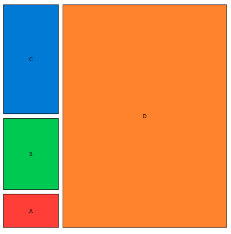
Typstonomicon, or The Code You Should Not Write
Totally cursed examples with lots of quires, measure and other things to hack around current Typst limitations. Generally you should use this code only if you really need it.
I think that this chapter will slowly die as Typst matures.
Word count
Recommended solution
Use wordometr package:
#import "@preview/wordometer:0.1.4": word-count, total-words
#show: word-count
In this document, there are #total-words words all up.
#word-count(total => [
The number of words in this block is #total.words
and there are #total.characters letters.
])
Just count all words in document
// original author: laurmaedje
#let words = counter("words")
#show regex("\p{L}+"): it => it + words.step()
== A heading
#lorem(50)
=== Strong chapter
#strong(lorem(25))
// it is ignoring comments
#align(right)[(#context words.display() words)]
Count only some elements, ignore others
// original author: jollywatt
#let count-words(it) = {
let fn = repr(it.func())
if fn == "sequence" { it.children.map(count-words).sum() }
else if fn == "text" { it.text.split().len() }
else if fn in ("styled") { count-words(it.child) }
else if fn in ("highlight", "item", "strong", "link") { count-words(it.body) }
else if fn in ("footnote", "heading", "equation") { 0 }
else { 0 }
}
#show: rest => {
let n = count-words(rest)
rest + align(right, [(#n words)])
}
== A heading (shouldn't be counted)
#lorem(50)
=== Strong chapter
#strong(lorem(25)) // counted too!
Try & Catch
// author: laurmaedje
// Renders an image or a placeholder if it doesn't exist.
// Don’t try this at home, kids!
#let maybe-image(path, ..args) = context {
let path-label = label(path)
let first-time = query((context {}).func()).len() == 0
if first-time or query(path-label).len() > 0 {
[#image(path, ..args)#path-label]
} else {
rect(width: 50%, height: 5em, fill: luma(235), stroke: 1pt)[
#set align(center + horizon)
Could not find #raw(path)
]
}
}
#maybe-image("../tiger.jpg")
#maybe-image("../tiger1.jpg")
Breakpoints on broken blocks
Implementation with table headers & footers
See a demo project (more comments, I stripped some of them) there.
/// author: isuffix
// Underlying counter and zig-zag functions
#let counter-family(id) = {
let parent = counter(id)
let parent-step() = parent.step()
let get-child() = counter(id + str(parent.get().at(0)))
return (parent-step, get-child)
}
// A fun zig-zag line!
#let zig-zag(fill: black, rough-width: 6pt, height: 4pt, thick: 1pt, angle: 0deg) = {
layout((size) => {
// Use layout to get the size and measure our horizontal distance
// Then get the per-zigzag width with some maths.
let count = int(calc.round(size.width / rough-width))
// Need to add extra thickness since we join with `h(-thick)`
let width = thick + (size.width - thick) / count
// One zig and one zag:
let zig-and-zag = {
let line-stroke = stroke(thickness: thick, cap: "round", paint: fill)
let top-left = (thick/2, thick/2)
let bottom-mid = (width/2, height - thick/2)
let top-right = (width - thick/2, thick/2)
let zig = line(stroke: line-stroke, start: top-left, end: bottom-mid)
let zag = line(stroke: line-stroke, start: bottom-mid, end: top-right)
box(place(zig) + place(zag), width: width, height: height, clip: true)
}
let zig-zags = ((zig-and-zag,) * count).join(h(-thick))
rotate(zig-zags, angle)
})
}
// ---- Define split-box ---- //
// Customizable options for a split-box border:
#let default-border = (
// The starting and ending lines
above: line(length: 100%),
below: line(length: 100%),
// Lines to put between the box over multiple pages
btwn-above: line(length: 100%, stroke: (dash:"dotted")),
btwn-below: line(length: 100%, stroke: (dash:"dotted")),
// Left/right lines
// These *must* use `grid.vline()`, otherwise you will get an error.
// To remove the lines, set them to: `grid.vline(stroke: none)`.
// You could probably configure this better with a rowspan, but I'm lazy.
left: grid.vline(),
right: grid.vline(),
)
// Create a box for content which spans multiple pages/columns and
// has custom borders above and below the column-break.
#let split-box(
// Set the border dictionary, see `default-border` above for options
border: default-border,
// The cell to place content in, this should resolve to a `grid.cell`
cell: grid.cell.with(inset: 5pt),
// The last positional arg or args are your actual content
// Any extra named args will be sent to the underlying grid when called
// This is useful for fill, align, etc.
..args
) = {
// See `utils.typ` for more info.
let (parent-step, get-child) = counter-family("split-box-unique-counter-string")
parent-step() // Place the parent counter once.
// Keep track of each time the header is placed on a page.
// Then check if we're at the first placement (for header) or the last (footer)
// If not, we'll use the 'between' forms of the border lines.
let border-above = context {
let header-count = get-child()
header-count.step()
context if header-count.get() == (1,) { border.above } else { border.btwn-above }
}
let border-below = context {
let header-count = get-child()
if header-count.get() == header-count.final() { border.below } else { border.btwn-below }
}
// Place the grid!
grid(
..args.named(),
columns: 3,
border.left,
grid.header(border-above , repeat: true),
..args.pos().map(cell),
grid.footer(border-below, repeat: true),
border.right,
)
}
// ---- Examples ---- //
#set page(width: 7.2in, height: 3in, columns: 6)
// Tada!
#split-box[
#lorem(20)
]
// And here's a fun example:
#let fun-border = (
// gradients!
above: line(length: 100%, stroke: 2pt + gradient.linear(..color.map.rainbow)),
below: line(length: 100%, stroke: 2pt + gradient.linear(..color.map.rainbow, angle: 180deg)),
// zig-zags!
btwn-above: move(dy: +2pt, zig-zag(fill: blue, angle: 3deg)),
btwn-below: move(dy: -2pt, zig-zag(fill: orange, angle: 177deg)),
left: grid.vline(stroke: (cap: "round", paint: purple)),
right: grid.vline(stroke: (cap: "round", paint: purple)),
)
#split-box(border: fun-border)[
#lorem(25)
]
// And some more tame friends:
#split-box(border: (
above: move(dy: -0.5pt, line(length: 100%)),
below: move(dy: +0.5pt, line(length: 100%)),
// zig-zags!
btwn-above: move(dy: -1.1pt, zig-zag()),
btwn-below: move(dy: +1.1pt, zig-zag(angle: 180deg)),
left: grid.vline(stroke: (cap: "round")),
right: grid.vline(stroke: (cap: "round")),
))[
#lorem(10)
]
#split-box(
border: (
above: line(length: 100%, stroke: luma(50%)),
below: line(length: 100%, stroke: luma(50%)),
btwn-above: line(length: 100%, stroke: (dash: "dashed", paint: luma(50%))),
btwn-below: line(length: 100%, stroke: (dash: "dashed", paint: luma(50%))),
left: grid.vline(stroke: none),
right: grid.vline(stroke: none),
),
cell: grid.cell.with(inset: 5pt, fill: color.yellow.saturate(-85%))
)[
#lorem(20)
]

Implementation via headers, footers and stated
#let countBoundaries(loc, fromHeader) = {
let startSelector = selector(label("boundary-start"))
let endSelector = selector(label("boundary-end"))
if fromHeader {
// Count down from the top of the page
startSelector = startSelector.after(loc)
endSelector = endSelector.after(loc)
} else {
// Count up from the bottom of the page
startSelector = startSelector.before(loc)
endSelector = endSelector.before(loc)
}
let startMarkers = query(startSelector)
let endMarkers = query(endSelector)
let currentPage = loc.position().page
let pageStartMarkers = startMarkers.filter(elem =>
elem.location().position().page == currentPage)
let pageEndMarkers = endMarkers.filter(elem =>
elem.location().position().page == currentPage)
(start: pageStartMarkers.len(), end: pageEndMarkers.len())
}
#set page(
margin: 2em,
// ... other page setup here ...
header: context {
let boundaryCount = countBoundaries(here(), true)
if boundaryCount.end > boundaryCount.start {
// Decorate this header with an opening decoration
[Block break top: $-->$]
}
},
footer: context {
let boundaryCount = countBoundaries(here(), false)
if boundaryCount.start > boundaryCount.end {
// Decorate this footer with a closing decoration
[Block break end: $<--$]
}
}
)
#let breakable-block(body) = block({
[
#metadata("boundary") <boundary-start>
]
stack(
// Breakable list content goes here
body
)
[
#metadata("boundary") <boundary-end>
]
})
#set page(height: 10em)
#breakable-block[
#([Something \ ]*10)
]

Extracting plain text
// original author: ntjess
#let stringify-by-func(it) = {
let func = it.func()
return if func in (parbreak, pagebreak, linebreak) {
"\n"
} else if func == smartquote {
if it.double { "\"" } else { "'" } // "
} else if it.fields() == (:) {
// a fieldless element is either specially represented (and caught earlier) or doesn't have text
""
} else {
panic("Not sure how to handle type `" + repr(func) + "`")
}
}
#let plain-text(it) = {
return if type(it) == str {
it
} else if it == [ ] {
" "
} else if it.has("children") {
it.children.map(plain-text).join()
} else if it.has("body") {
plain-text(it.body)
} else if it.has("text") {
if type(it.text) == str {
it.text
} else {
plain-text(it.text)
}
} else {
// remove this to ignore all other non-text elements
stringify-by-func(it)
}
}
#plain-text(`raw inline text`)
#plain-text(highlight[Highlighted text])
#plain-text[List
- With
- Some
- Elements
+ And
+ Enumerated
+ Too
]
#plain-text(underline[Underlined])
#plain-text($sin(x + y)$)
#for el in (
circle,
rect,
ellipse,
block,
box,
par,
raw.with(block: true),
raw.with(block: false),
heading,
) {
plain-text(el(repr(el)))
linebreak()
}
// Some empty elements
#plain-text(circle())
#plain-text(line())
#for spacer in (linebreak, pagebreak, parbreak) {
plain-text(spacer())
}
Horizontally align something with something
// author: tabiasgeehuman
#let inline-with(select, content) = context {
let target = query(
selector(select)
).last().location().position().x
let current = here().position().x
box(inset: (x: target - current + 0.3em), content)
}
#let inline-label(name) = [#line(length: 0%) #name]
#inline-with(selector(<start-c>))[= Common values]
#align(left, box[$
#inline-label(<start-c>) "Circles"(0) =& 0 \
lim_(x -> 1) "Circles"(0) =& 0
$])
Create zero-level chapters
// author: tinger
#let chapter = figure.with(
kind: "chapter",
// same as heading
numbering: none,
// this cannot use auto to translate this automatically as headings can, auto also means something different for figures
supplement: "Chapter",
// empty caption required to be included in outline
caption: [],
)
// emulate element function by creating show rule
#show figure.where(kind: "chapter"): it => {
set text(22pt)
counter(heading).update(0)
if it.numbering != none { strong(it.counter.display(it.numbering)) } + [ ] + strong(it.body)
}
// no access to element in outline(indent: it => ...), so we must do indentation in here instead of outline
#show outline.entry: it => {
if it.element.func() == figure {
// we're configuring chapter printing here, effectively recreating the default show impl with slight tweaks
let res = link(it.element.location(),
// we must recreate part of the show rule from above once again
if it.element.numbering != none {
numbering(it.element.numbering, ..it.element.counter.at(it.element.location()))
} + [ ] + it.element.body
)
if it.fill != none {
res += [ ] + box(width: 1fr, it.fill) + [ ]
} else {
res += h(1fr)
}
res += link(it.element.location(), it.page())
strong(res)
} else {
// we're doing indenting here
h(1em * it.level) + it
}
}
// new target selector for default outline
#let chapters-and-headings = figure.where(kind: "chapter", outlined: true).or(heading.where(outlined: true))
//
// start of actual doc prelude
//
#set heading(numbering: "1.")
// can't use set, so we reassign with default args
#let chapter = chapter.with(numbering: "I")
// an example of a "show rule" for a chapter
// can't use chapter because it's not an element after using .with() anymore
#show figure.where(kind: "chapter"): set text(red)
//
// start of actual doc
//
// as you can see these are not elements like headings, which makes the setup a bit harder
// because the chapters are not headings, the numbering does not include their chapter, but could using a show rule for headings
#outline(target: chapters-and-headings)
#chapter[Chapter]
= Chap Heading
== Sub Heading
#chapter[Chapter again]
= Chap Heading
= Chap Heading
== Sub Heading
=== Sub Sub Heading
== Sub Heading
#chapter[Chapter yet again]
Make all math display math
// author: eric1102
#show math.equation: it => {
if it.body.fields().at("size", default: none) != "display" {
return math.display(it)
}
it
}
Inline math: $sum_(n=0)^oo e^(x^2 - n/x^2)$\
Some other text on new line.
$
sum_(n=0)^oo e^(x^2 - n/x^2)
$
Empty pages without numbering
Empty pages before chapters starting at odd pages
// author: janekfleper
#set page(height: 20em)
#let find-labels(name) = {
return query(name).map(label => label.location().page())
}
#let page-header = context {
let empty-pages = find-labels(<empty-page>)
let new-chapters = find-labels(<new-chapter>)
if new-chapters.len() > 0 {
if new-chapters.contains(here().page()) [
_a new chapter starts on this page_
#return
]
// get the index of the next <new-chapter> label
let new-chapter-index = new-chapters.position(page => page > here().page())
if new-chapter-index != none {
let empty-page = empty-pages.at(new-chapter-index)
if empty-page < here().page() [
_this is an empty page to make the next chapter start on an odd page_
#return
]
}
}
[and this would be a regular header]
line(length: 100%)
}
#let page-footer = context {
// since the page breaks in chapter-heading() are inserted after the <empty-page> label,
// the selector has to look "before" the current page to find the relevant label
let empty-page-labels = query(selector(<empty-page>).before(here()))
if empty-page-labels.len() > 0 {
let empty-page = empty-page-labels.last().location().page()
// look back at the most recent <new-chapter> label
let new-chapter = query(selector(<new-chapter>).before(here())).last().location().page()
// check that there is no <new-chapter> label on the current page
if (new-chapter != here().page()) and (empty-page + 1 == here().page()) [
_this is an empty page where the page number should be omitted_
#return
]
}
let page-display = counter(page).display(here().page-numbering())
h(1fr) + page-display + h(1fr)
}
#show heading.where(level: 1): it => [
#[] <empty-page>
#pagebreak(to: "even", weak: true)
#[] <new-chapter>
#pagebreak(to: "odd", weak: true)
#it.body
#v(2em)
]
#show outline.entry.where(level: 1): it => {
// reverse the results of the label queries to find the last <empty-page> label for the targeted page
// the method array.position() will always return the first one...
let empty-pages = find-labels(<empty-page>).rev()
let new-chapters = query(<new-chapter>).rev()
let empty-page-index = empty-pages.position(page => page == int(it.page.text))
let new-chapter = new-chapters.at(empty-page-index)
link(new-chapter.location())[#it.body #box(width: 1fr)[#it.fill] #new-chapter.location().page()]
}
#set page(header: page-header, footer: page-footer, numbering: "1")
#outline()
= The explanation
```
These queries reveal where the corresponding tags are found. The actual empty page is always at the location of the label <empty-page> + 1. If an empty page is actually inserted by the pagebreaks, the two labels will cover the page of the heading and one page before that. If no empty page was inserted, both labels will point to the same page which is not an issue either. And even then we can check for the <new-chapter> label first to give it a higher priority.
The first <empty-page> label is always on page 1 and can just be ignored since it points to the (non-existing) empty page before the first chapter.
pages with the label <empty-page>: #context find-labels(<empty-page>)
pages with the label <new-chapter>: #context find-labels(<new-chapter>)
```
= A heading
#lorem(190)
= Another heading
#lorem(100)
= The last heading
#lorem(400)Multiple show rules
Sometimes there is a need to apply several rules that look very similar. Or generate them from code. One of the ways to deal with this, the most cursed one, is this:
#let rules = (math.sum, math.product, math.root)
#let apply-rules(rules, it) = {
if rules.len() == 0 {
return it
}
show rules.pop(): math.display
apply-rules(rules, it)
}
$product/sum root(3, x)/2$
#show: apply-rules.with(rules)
$product/sum root(3, x)/2$
The recursion problem may be avoided with the power of fold, with basically the same idea:
// author: Eric
#let kind_supp = (code: "Listing", algo: "Algorithme")
#show: it => kind_supp.pairs().fold(it, (acc, (kind, supp)) => {
show figure.where(kind: kind): set figure(supplement: supp)
acc
})
Note that just in case of symbols (if you don't need element functions), one can use regular expressions. That is a more robust way:
#show regex("[" + math.product + math.sum + "]"): math.display
$product/sum root(3, x)/2$
Remove indent from nested lists
// author: fenjalien
#show enum.item: it => {
if repr(it.body.func()) == "sequence" {
let children = it.body.children
let index = children.position(x => x.func() == enum.item)
if index != none {
enum.item({
children.slice(0, index).join()
set enum(indent: -1.2em) // Note that this stops an infinitly recursive show rule
children.slice(index).join()
})
} else {
it
}
} else {
it
}
}
arst
+ A
+ b
+ c
+ d
+ e
+ f
+ g
+ h
+ i
+ 